This is a follow-on to Why Does Biological Evolution Work? A Minimal Model for Biological Evolution and Other Adaptive Processes [May 3, 2024].
Even More from an Extremely Simple Model
A few months ago I introduced an extremely simple “adaptive cellular automaton” model that seems to do remarkably well at capturing the essence of what’s happening in biological evolution. But over the past few months I’ve come to realize that the model is actually even richer and deeper than I’d imagined. And here I’m going to describe some of what I’ve now figured out about the model—and about the often-surprising things it implies for the foundations of biological evolution.
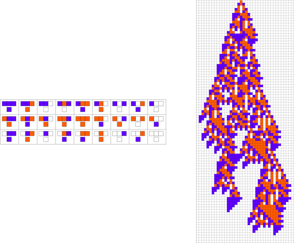
The starting point for the model is to view biological systems in abstract computational terms. We think of an organism as having a genotype that’s represented by a program, that’s then run to produce its phenotype. So, for example, the cellular automaton rules on the left correspond to a genotype which are then run to produce the phenotype on the right (starting from a “seed” of a single red cell):
The key idea in our model is to adaptively evolve the genotype rules—say by making single “point mutations” to the list of outcomes from the rules:
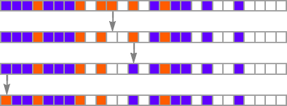
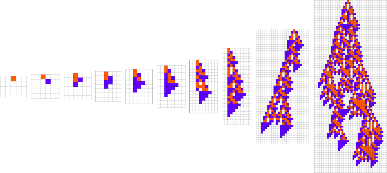
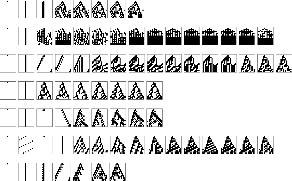
At each step in the adaptive evolution we “accept” a mutation if it leads to a phenotype that has a higher—or at least equal—fitness relative to what we had before. So, for example, taking our fitness function to be the height (i.e. lifetime) of the phenotype pattern (with patterns that are infinite being assigned zero fitness), a sequence of (randomly chosen) adaptive evolution steps that go from the null rule to the rule above might be:
What if we make a different sequence of randomly chosen adaptive evolution steps? Here are a few examples of what happens—each in a sense “using a different idea” for how to achieve high fitness:
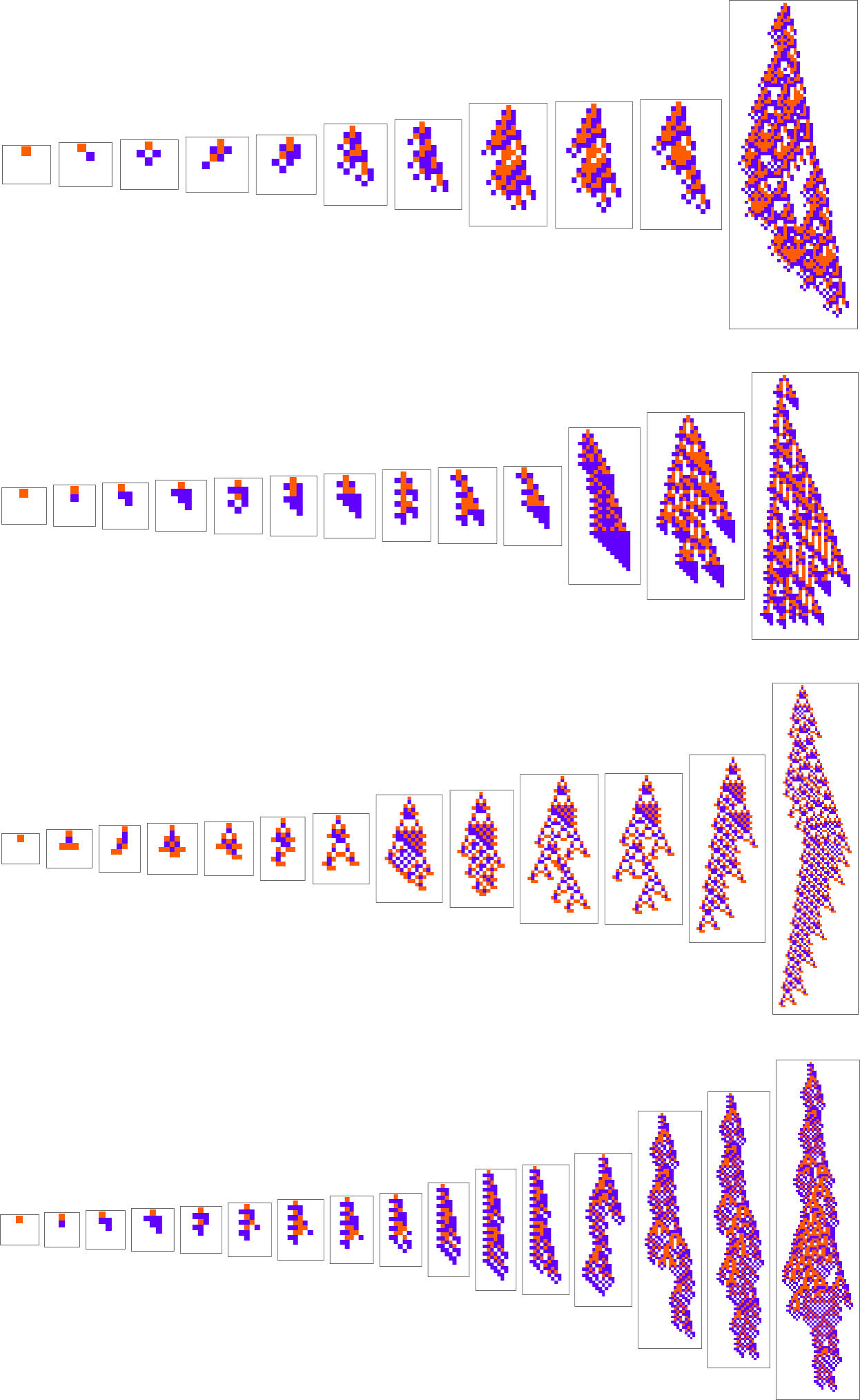
And, yes, one can’t help but be struck by how “lifelike” this all looks—both in the complexity of these patterns, and in their diversity. But what is ultimately responsible for what we’re seeing? It’s long been a core question about biological evolution. Are the forms it produces the result of careful “sculpting” by the environment (and by the fitness functions it implies)—or are their most important features somehow instead a consequence of something more intrinsic and fundamental that doesn’t depend on details of fitness functions?
Well, let’s say we pick a different fitness function—for example, not the height of a phenotype pattern, but instead its width (or, more specifically, the width of its bounding box). Here are some results of adaptive evolution in this case:
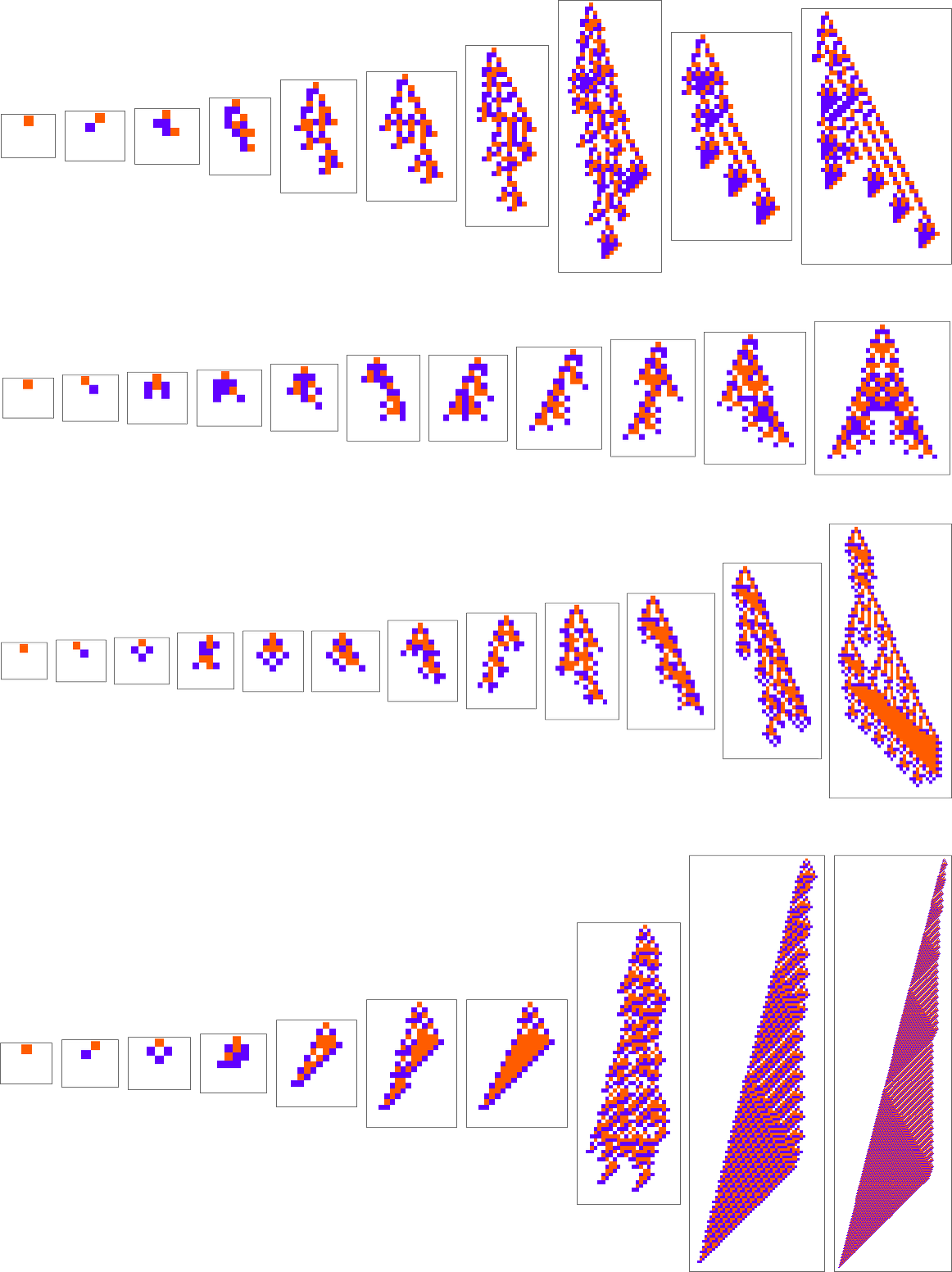
And, yes, the patterns we get are now ones that achieve larger “bounding box width”. But somehow there’s still a remarkable similarity to what we saw with a rather different fitness function above. And, for example, in both cases, high fitness, it seems, is normally achieved in a complicated and hard-to-understand way. (The last pattern is a bit of an exception; as can also happen in biology, this is a case where for once there’s a “mechanism” in evidence that we can understand.)
So what in the end is going on? As I discussed when I introduced the model a few months ago, it seems that the “dominant force” is not selection according to fitness functions, but instead the fundamental computational phenomenon of computational irreducibility. And what we’ll find here is that in fact what we see is, more than anything, the result of an interplay between the computational irreducibility of the process by which our phenotypes develop, and the computational boundedness of typical forms of fitness functions.
The importance of such an interplay is something that’s very much come into focus as a result of our Physics Project. And indeed it now seems that the foundations of both physics and mathematics are—more than anything—reflections of this interplay. And now it seems that’s true of biological evolution as well.
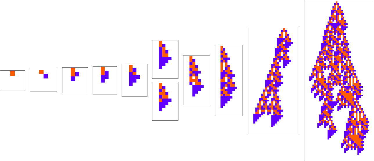
In studying our model, there are many detailed phenomena we’ll encounter—most of which seem to have surprisingly direct analogs in actual biological evolution. For example, here’s what happens if we plot the behavior of the fitness function for our first example above over the course of the adaptive evolution process:
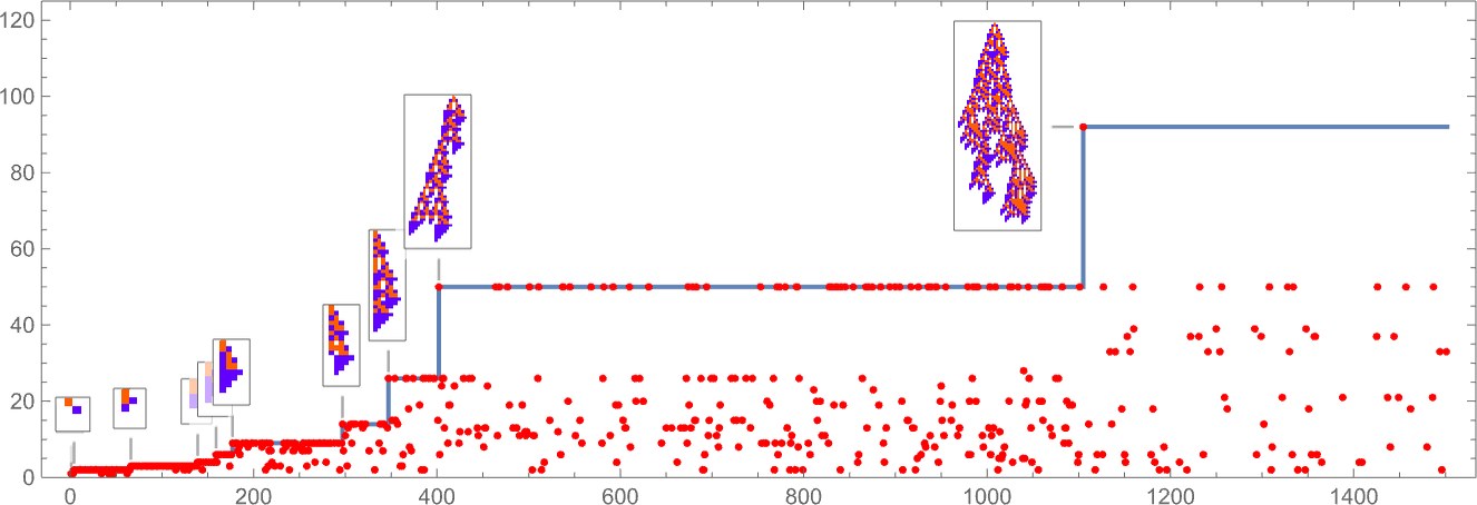
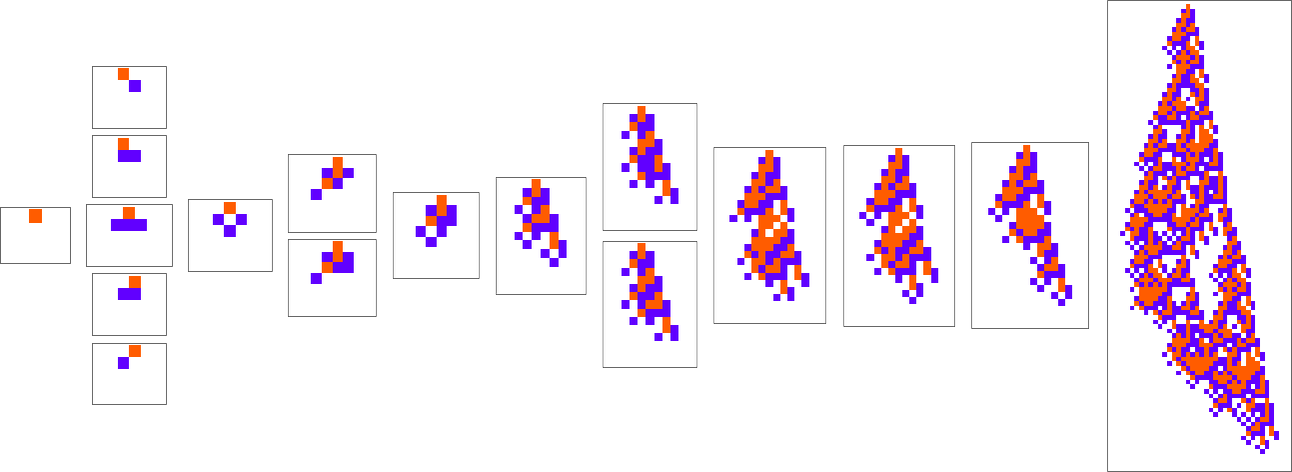
We see a sequence of “plateaus”, punctuated by jumps in fitness that reflect some “breakthrough” being made. In the picture, each red dot represents the fitness associated with a genotype that was tried. Many fall below the line of “best results so far”. But there are also plenty of red dots that lie right on the line. And these correspond to genotypes that yield the same fitness that’s already been achieved. But here—as in actual biological evolution—it’s important that there can be “fitness-neutral evolution”, where genotypes change, but the fitness does not. Usually such changes of genotype yield not just the same fitness, but also the exact same phenotype. Sometimes, however, there can be multiple phenotypes with the same fitness—and indeed this happens at one stage in the example here
and at multiple stages in the second example we showed above:
The Multiway Graph of All Possible Evolutions
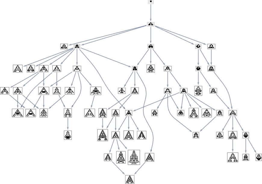
In the previous section we saw examples of the results of a few particular random sequences of mutations. But what if we were to look at all possible sequences of mutations? As I discussed when I introduced the model, it’s possible to construct a multiway graph that represents all possible mutation paths. Here’s what one gets for symmetric k = 2, r = 2 rules—starting from the null rule, and using height as a fitness function:
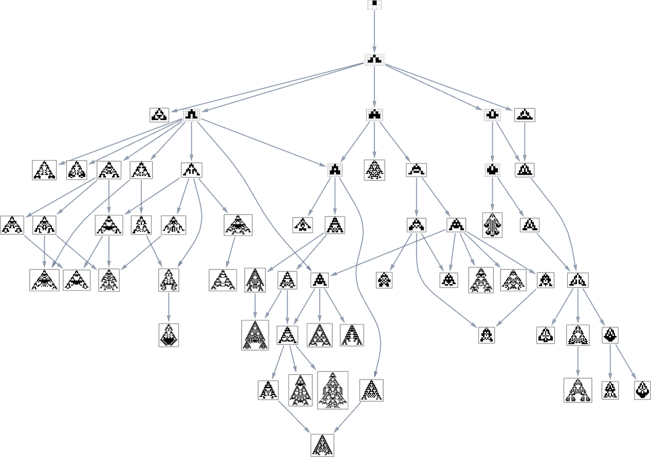
The way this graph is constructed, there are arrows from a given phenotype to all phenotypes with larger (finite) height that can be reached by a single mutation.
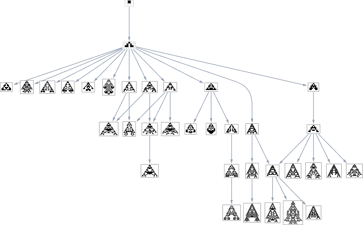
But what if our fitness function is width rather than height? Well, then we get a different multiway graph in which arrows go to phenotypes not with larger height but instead with larger width:
So what’s really going on here? Ultimately one can think of there being an underlying graph (that one might call the “mutation graph”) in which every edge represents a transformation between two phenotypes that can be achieved by a single mutation in the underlying genotype:
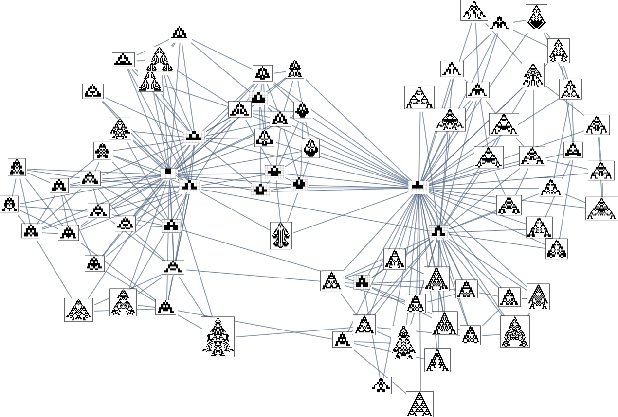
At this level, the transformations can go either way, so this graph is undirected. But the crucial point is that as soon as one imposes a fitness function, it defines a particular direction for each transformation (at least, each transformation that isn’t fitness neutral for this fitness function). And then if one starts, say, from the null rule, one will pick out a certain “evolution cone” subgraph of the original mutation graph.
So, for example, with width as the fitness function, the subgraph one gets is what’s highlighted here:
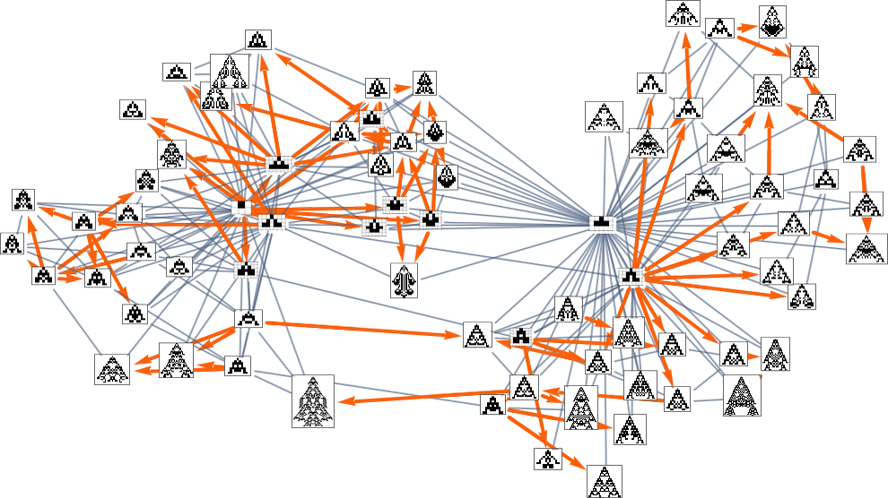
There are several subtleties here. First, we simplified the multiway graph by doing transitive reduction and drawing only the minimal edges necessary to define the connectivity of the graph. If we want to see all possible single-mutation transformations between phenotypes we need to do transitive completion, in which case for the width fitness function the multiway graph we get is:
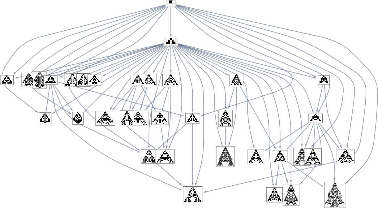
But now there’s another subtlety. The edges in the multiway graph represent fitness-changing transformations. But there are also fitness-neutral transformations. And occasionally these can even lead to different (though equal-fitness) phenotypes, so that really each node in the graph above (say, the transitively reduced one) should sometimes be associated with multiple phenotypes
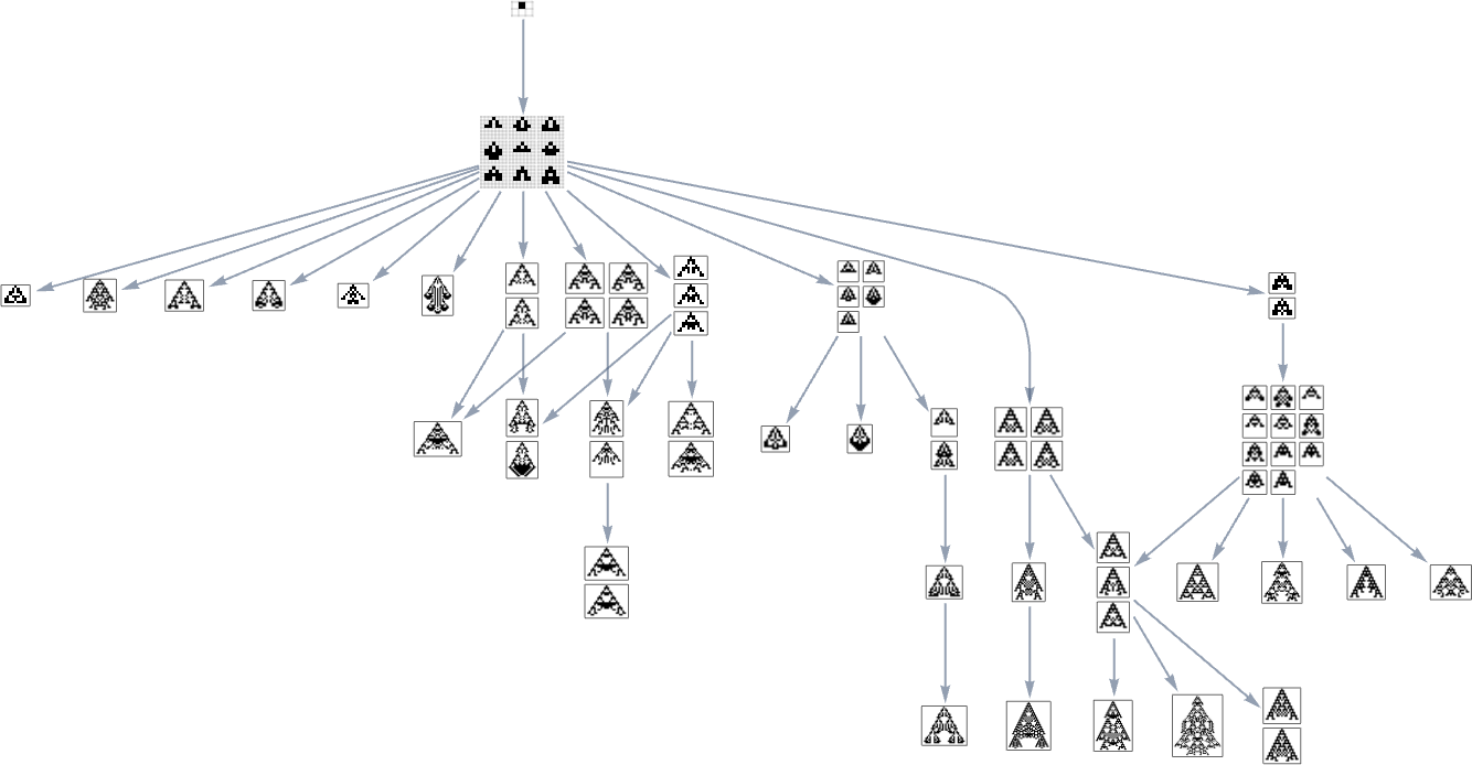
which can “fitness neutrally” transform into each other, as in:
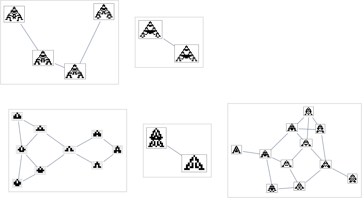
But even this isn’t the end of the subtleties. Fitness-neutral sets typically contain many genotypes differing by changes of rule cases that don’t affect the phenotype they produce. But it may be that just one or a few of these genotypes are “primed” to be able to generate another phenotype with just one additional mutation. Or, in other words, each node in the multiway graph above represents a whole class of genotypes “equivalent under fitness-neutral transformations”, and when we draw an arrow it indicates that some genotype in that class can be transformed by a single mutation to some genotype in the class associated with a different phenotype:

But beyond the subtleties, the key point is that particular fitness functions in effect just define particular orderings on the underlying mutation graph. It’s somewhat like choices of reference frames or families of simultaneity surfaces in physics. Different choices of fitness function in effect define different ways in which the underlying mutation graph can be “navigated” by evolution over the course of time.
As it happens, the results are not so different between height and width fitness functions. Here’s a combined multiway graph, indicating transformations variously allowed by these different fitness functions:
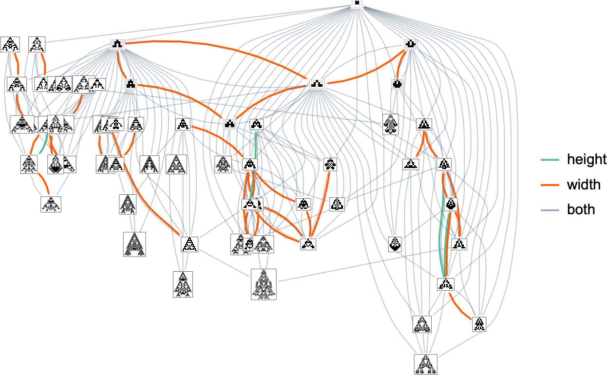
Homing in on a small part of this graph, we see that there are different “flows” associated with maximizing height and maximizing width:
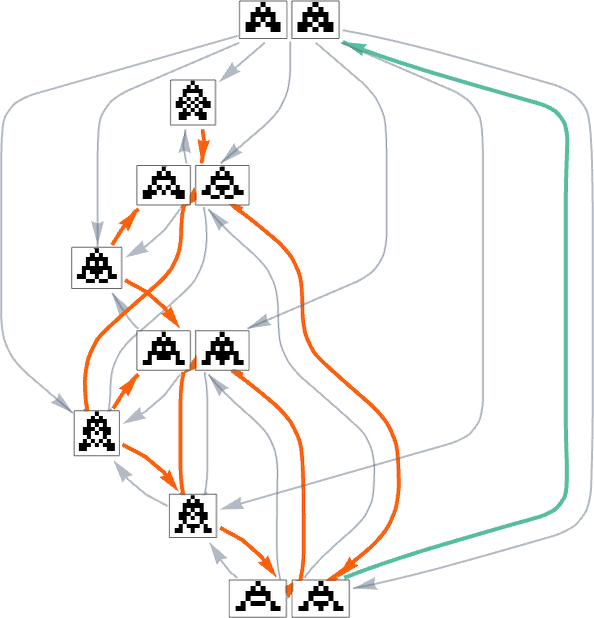
With a single fitness function that for any two phenotypes systematically treats one phenotype as fitter than another, the multiway graph must always define a definite flow. But as soon as one considers changing fitness functions in the course of evolution, it’s possible to get cycles in the multiway graph, as in the example above—so that, in effect, “evolution can repeat itself”.
Fitness Functions Based on Aspect Ratio
We’ve looked at fitness functions based on maximizing height and on maximizing width. But what if we try to combine these? Here’s a plot of the widths and heights of all phenotypes that occur in the symmetric k = 2, r = 2 case we studied above:
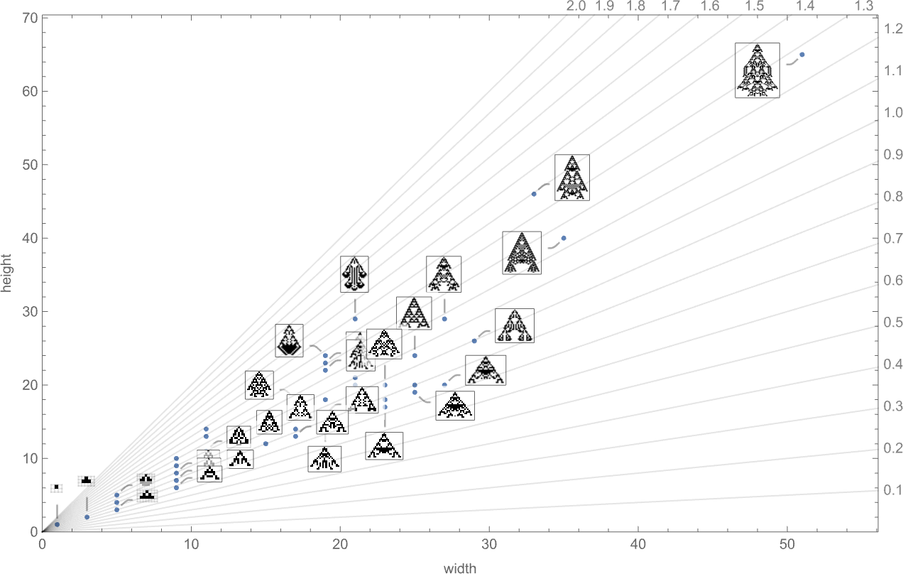
We could imagine a variety of ways to define “fitness frontiers” here. But as a specific example, let’s consider fitness functions that are based on trying to achieve specific aspect ratios—i.e. phenotypes that are as close as possible to a particular constant-aspect-ratio line in the plot above.
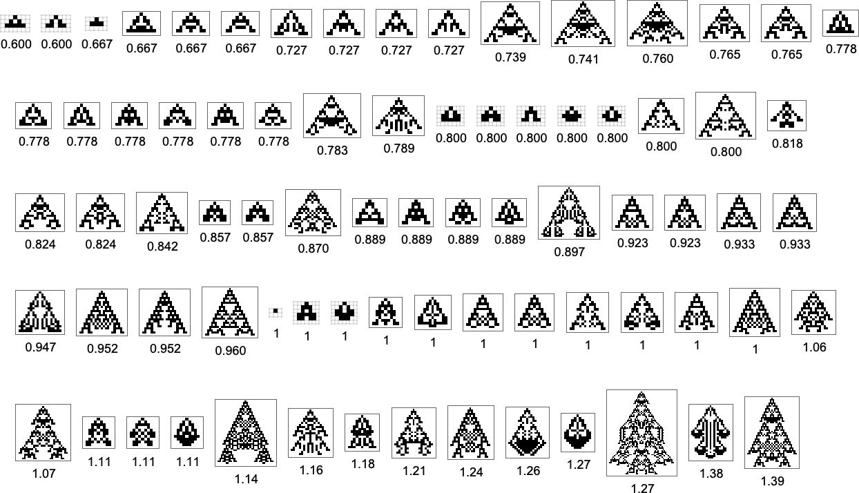
With the symmetric k = 2, r = 2 rules we’re using here, only a certain set of aspect ratios can ever be obtained:


The corresponding phenotypes (with their aspect ratios) are:
As we change the aspect ratio that we’re trying to achieve, the evolution multiway graph will change:
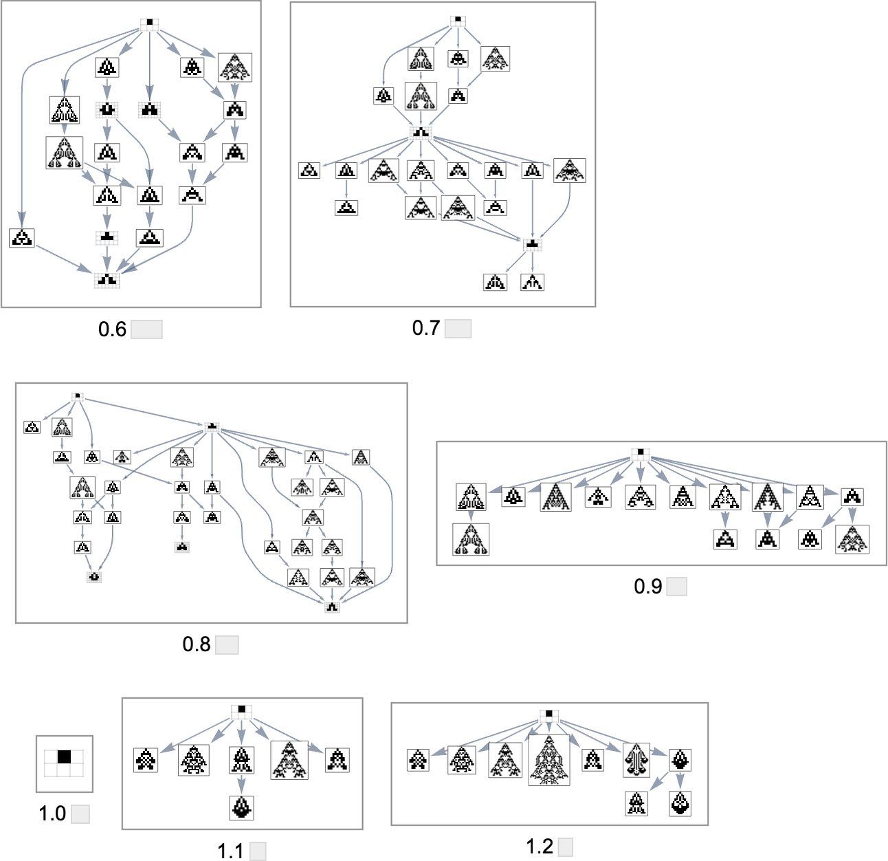
In all cases we’re starting from the null rule. For target aspect ratio 1.0 this rule itself already achieves that aspect ratio—so the multiway graph in that case is trivial. But in general, different aspect ratios yield evolution multiway graphs that are different subgraphs of the complete mutation graph we saw above.
So if we follow all possible paths of evolution, how close can we actually get to any given target aspect ratio? This plot shows what final aspect ratios can be achieved as a function of target aspect ratio:
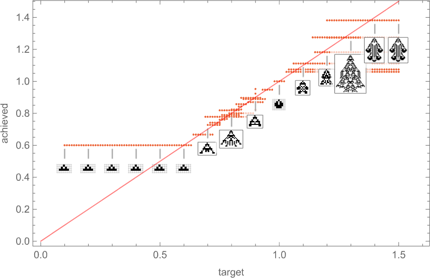
And in a sense this is a summary of the effect of “developmental constraints” for “adaptive cellular automaton organisms” like this. If there were no constraints then for every target aspect ratio it’d be possible to get an “organism” with that aspect ratio—so in the plot there’d be a point lying on the red line. But in actuality the process of cellular automaton growth imposes constraints—that in particular allows only certain phenotypes, with certain aspect ratios, to exist. And beyond that, which phenotypes can actually be reached by adaptive evolution depends on the evolution multiway graph, with “different turns” on the graph leading to different fitness (i.e. different aspect ratio) phenotypes.
But what the plot above shows overall is that for a certain range of target aspect ratios, adaptive evolution is successfully able to get at least close to those aspect ratios. If the target aspect ratio gets out of that range, however, “developmental constraints” come in that prevent the target from being reached.
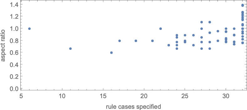
With “larger genomes”, i.e. rules with larger numbers of cases to specify, it’s possible to do better, and to more accurately achieve particular aspect ratios, over larger ranges of values. And indeed we can see some version of this effect even for symmetric k = 2, r = 2 rules by plotting aspect ratios that can be achieved as a function of the number of cases that need to be specified in the rule:
As an alternative visualization, we can plot the “best convergence to the target” as a function of the number of rule cases—and once again we see that larger numbers of rule cases let us get closer to target aspect ratios:

It’s worth mentioning that—just as we discussed for height and width fitness functions above—there are subtleties here associated with fitness-neutral sets. For example, here are sets of phenotypes that all have the specified aspect ratios—with phenotypes that can be reached by single point mutations being joined:

In the evolution multiway graphs above, we included only one phenotype for each fitness-neutral set. But here’s what we get for target aspect ratio 0.7 if we show all phenotypes with a given fitness:
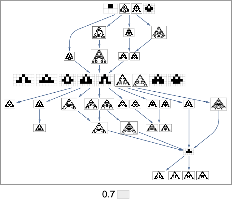
Note that on the top line, we don’t just get the null rule. Instead, we get four phenotypes, all of which, like the null rule, have aspect ratio 1, and so are equally far from the target aspect ratio 0.7.
The picture above is only the transitively reduced graph. But if we include all possible transformations associated with single point mutations, we get instead:
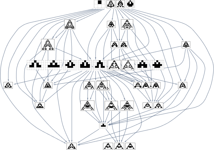
Based on this graph, we can now make what amounts to a foliation, showing collections of phenotypes reached by a certain minimum number of mutations, progressively approaching our target aspect ratio (here 0.7):
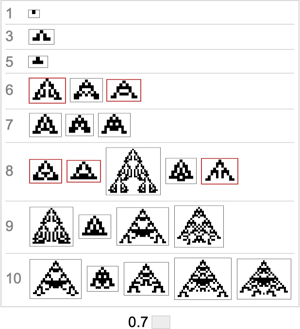
Here’s what we get from the range of target aspect ratios shown above (where, as above, “terminal phenotypes” are highlighted):
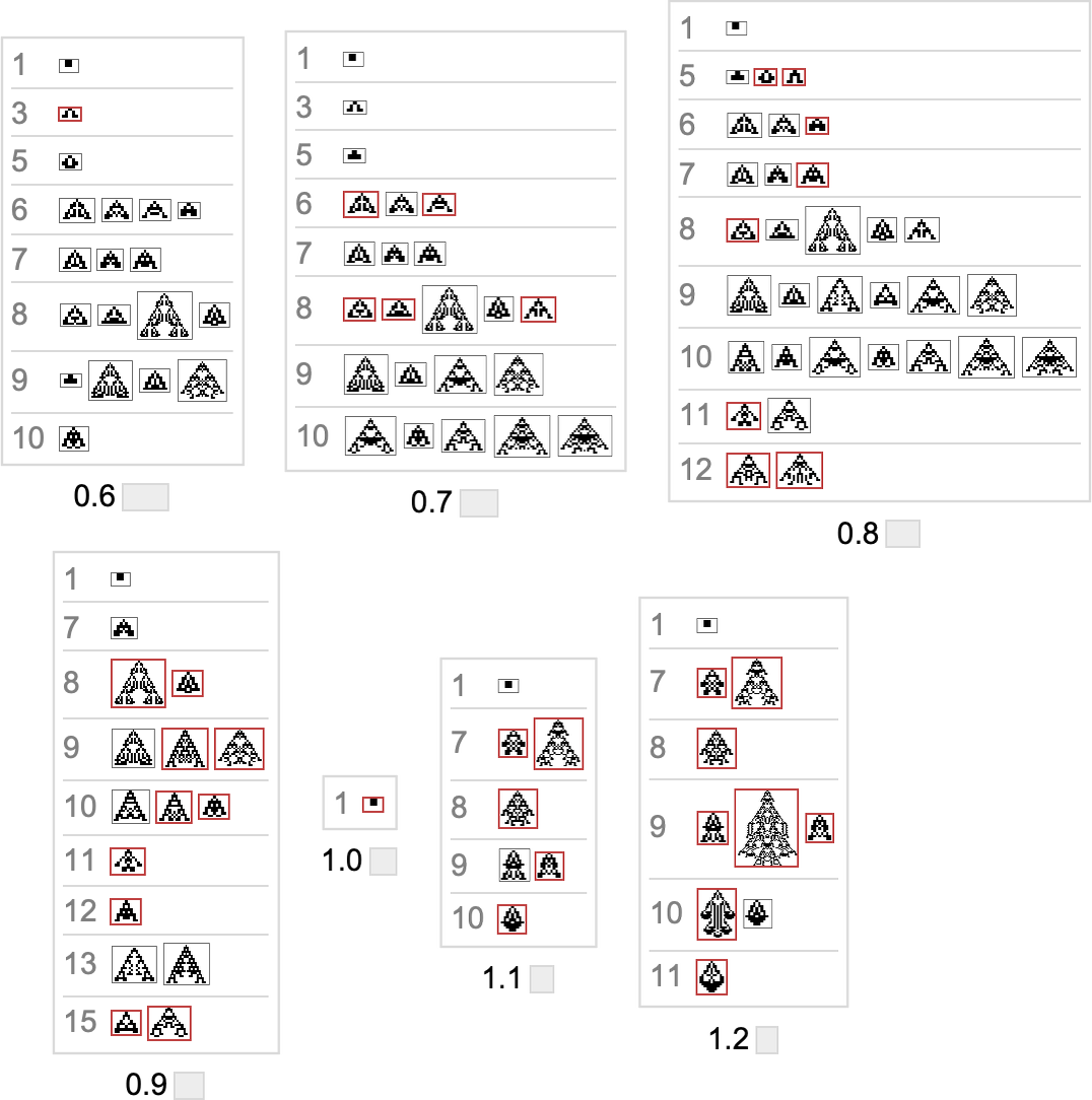
In a sense these sequences show us what phenotypes can appear at progressive stages in the “fossil record” for different (aspect-ratio) fitness functions in our very simple model. The highlighted cases are “evolutionary dead ends”. The others can evolve further.
Unreachable Cases
Our model takes the process of adaptive evolution to never “go backwards”, or, in other words, to never evolve from a particular genotype to one with lower fitness. But this means that starting with a certain genotype (say the null rule) there may be genotypes (and hence phenotypes) that will never be reached.
With height as a fitness function, there are just two single (“orphan”) phenotypes that can’t be reached:
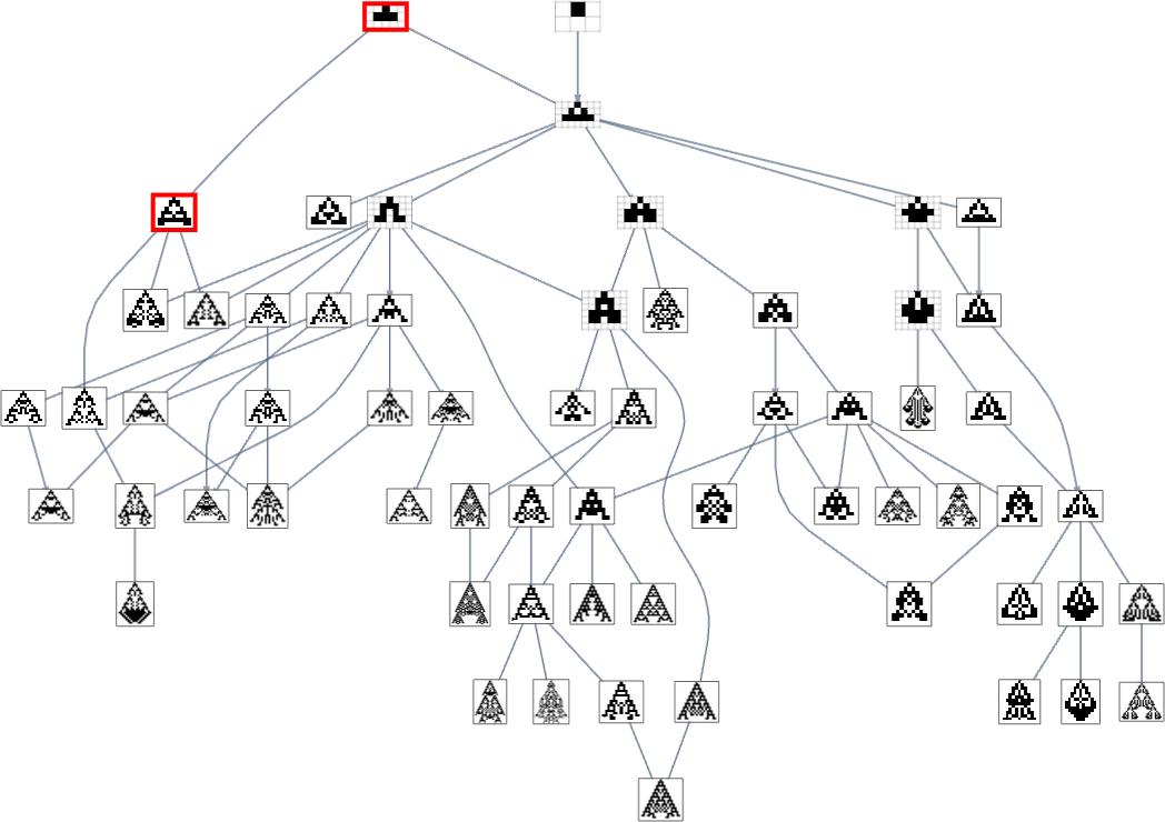
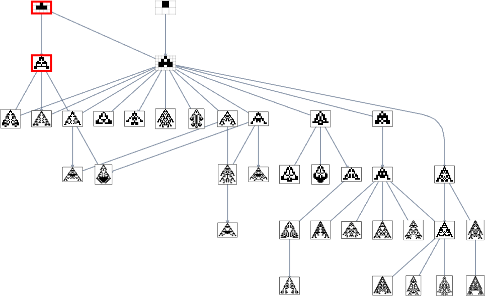
And with width as the fitness function, it turns out the very same phenotypes also can’t be reached:
But if we use a fitness function that, for example, tries to achieve aspect ratio 0.7, we get many more phenotypes that can’t be reached starting from the null rule:
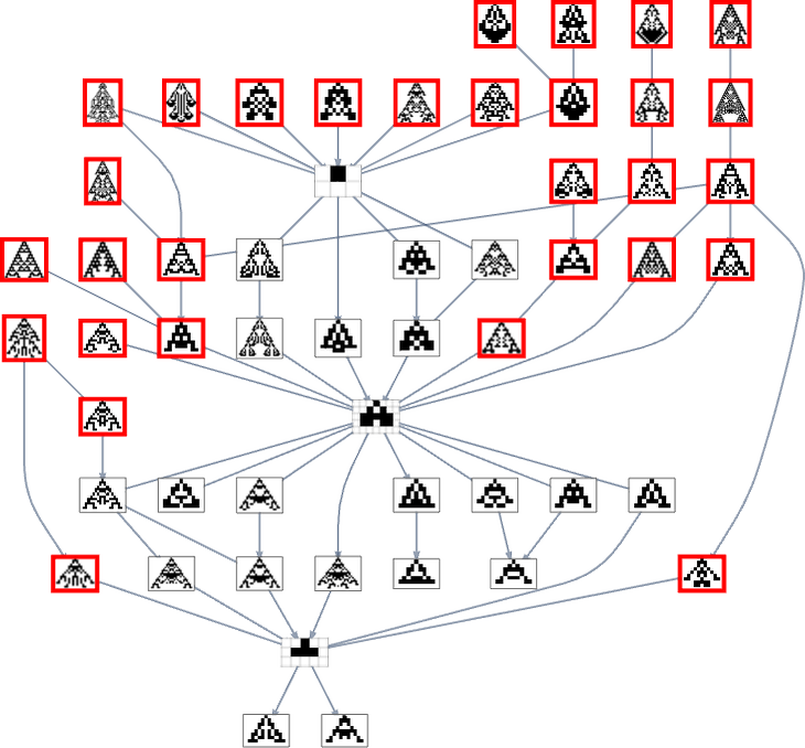
In the original mutation graph all the phenotypes appear. But when we foliate (or, more accurately, order) that graph using a particular fitness function, some phenotypes become unreachable by evolutionarily-possible transformations—in a rough analogy to the way some events in physics can become unreachable in the presence of an event horizon.
Multiway Graphs for Larger Rule Spaces
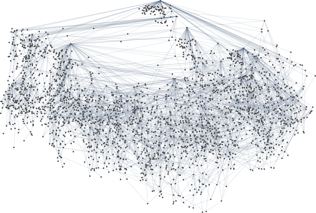
So far we’ve discussed multiway graphs here only for symmetric k = 2, r = 2 rules. There are a total of 524,288 (= 219) possible such rules, producing 77 distinct phenotypes. But what about larger classes of rules? As an example, we can consider all k = 2, r = 2 rules, without the constraint of symmetry. There are 2,147,483,648 (= 231) possible such rules, and there turn out to be 3137 distinct phenotypes.
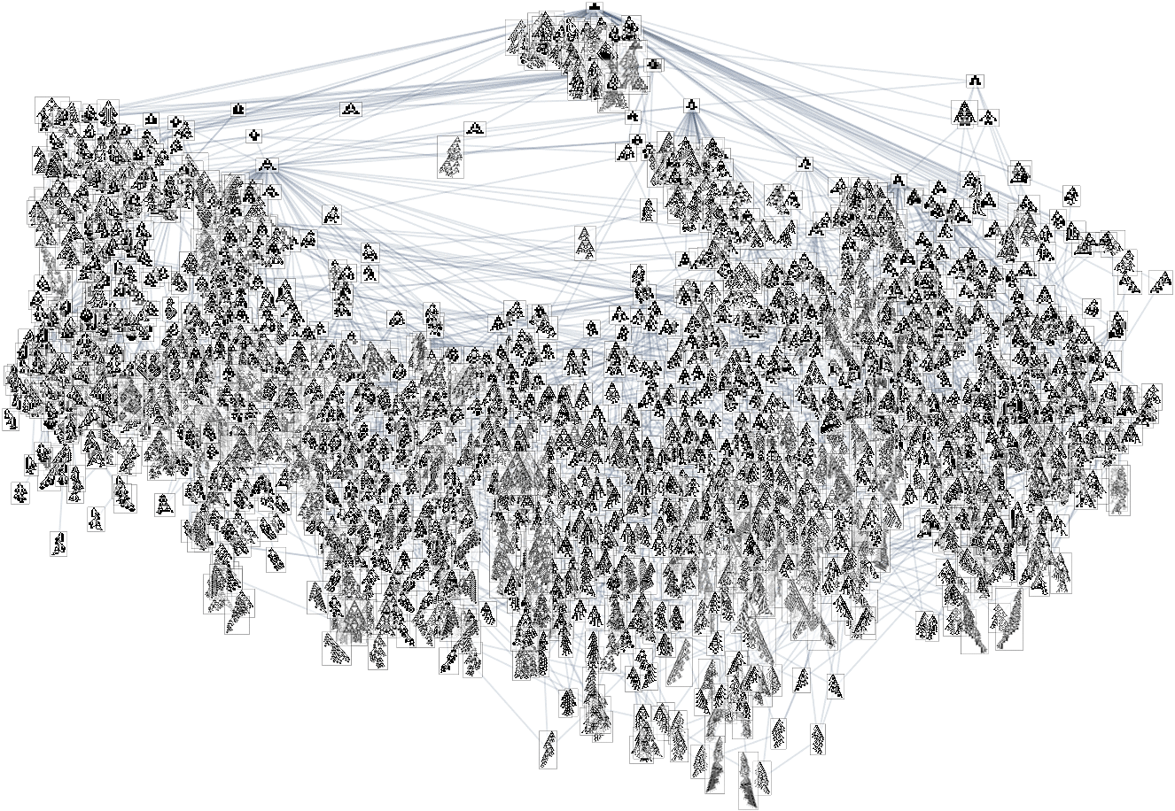
For the height fitness function, the complete multiway graph in this case is
or, annotated with actual phenotypes:
If instead we just show bounding boxes, it’s easier to see where long-lifetime phenotypes occur:
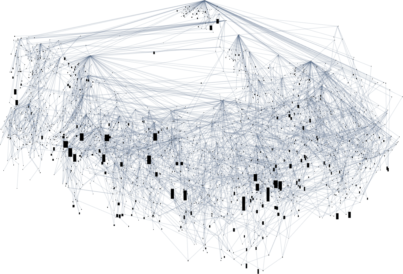
With a different graph layout the evolution multiway graph (with initial node indicated) becomes:
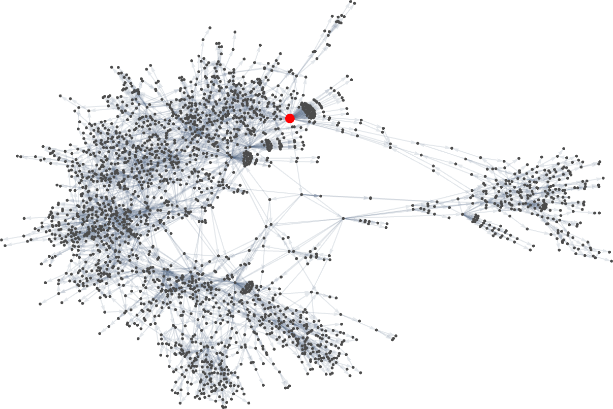
One subtlety here is that the null rule has no successors with single point mutation. When we were talking about symmetric k = 2, r = 2 rules, we took a “single point mutation” always to change both a particular rule case and its mirror image. But if we don’t have the symmetry requirement, a single point mutation really can just change a single rule case. And if we start from the null range and look at the results of changing just one bit (i.e. the output of just one rule case) in all possible ways we find that we either get the same pattern as with the null rule, or we get a pattern that grows without bound:

Or, put another way, we can’t get anywhere with single bit mutations starting purely from the null rule. So what we’ve done is instead to start our multiway graph from k = 2, r = 2 rule 20, which has two bits “on”, and gives phenotype:

But starting from this, just one mutation (together with a sequence of fitness-neutral mutations) is sufficient to give 94 phenotypes—or 49 after removing mirror images:

The total number of new phenotypes we can reach after successively more (non-fitness-neutral) mutations is

while the successive longest-lifetime patterns are:
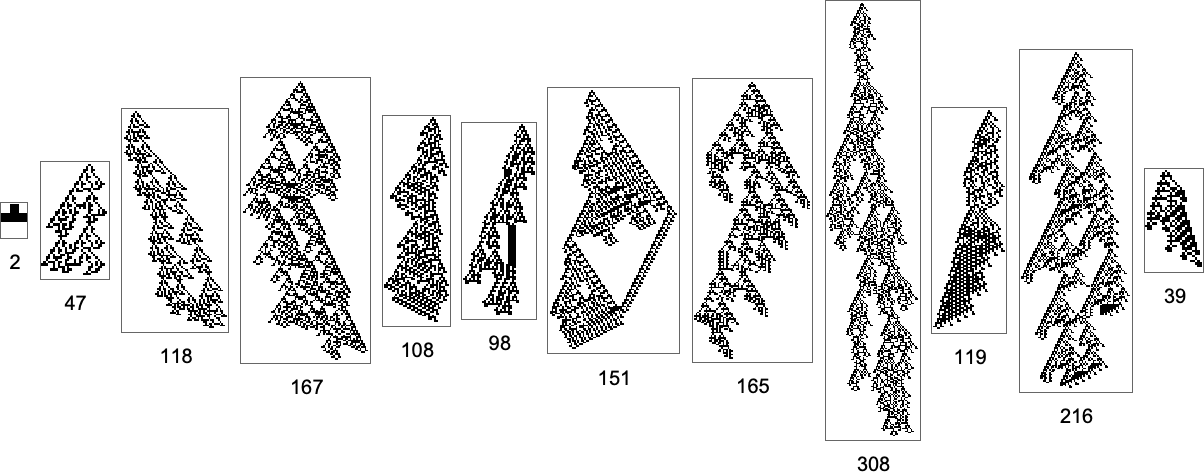
And what we see here is that it’s in principle possible to achieve long lifetimes even with fairly few mutations. But when the mutations are done at random, it can still take a very large number of steps to successfully “random walk” to long lifetime phenotypes.
And out of a total of 2407 distinct phenotypes, 984 are “dead ends” where no further evolution is possible. Some of these dead ends have long lifetimes

but others have very short lifetimes:

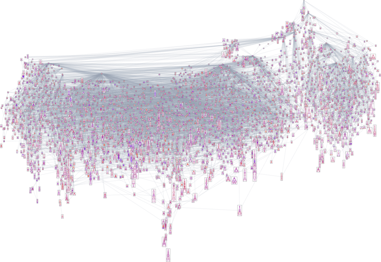
There’s much more to explore in this multiway graph—and we’ll continue a bit below. But for now let’s look at another evolution multiway graph of accessible size: the one for symmetric k = 3, r = 1 rules. There are a total of 129,140,163 (= 317) possible such rules, that yield a total of 14,778 distinct phenotypes:
Showing only bounding boxes of patterns this becomes:
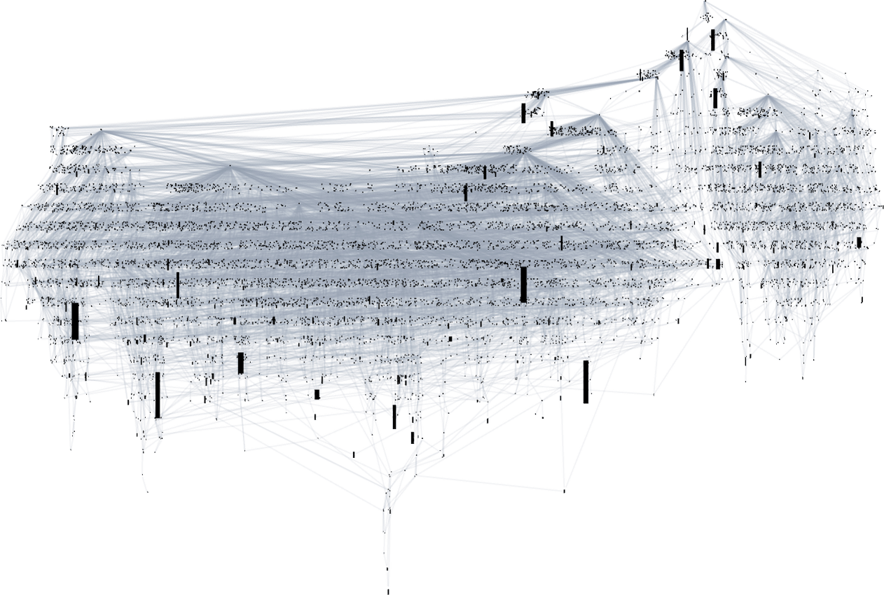
Unlike the k = 2, r = 2 case, we can now start this whole graph with the null rule. However, if we look at all possible symmetric k = 3, r = 1 rules, there turn out to be 6 “isolates” that can’t be reached from the null rule by adaptive evolution with the height fitness function:
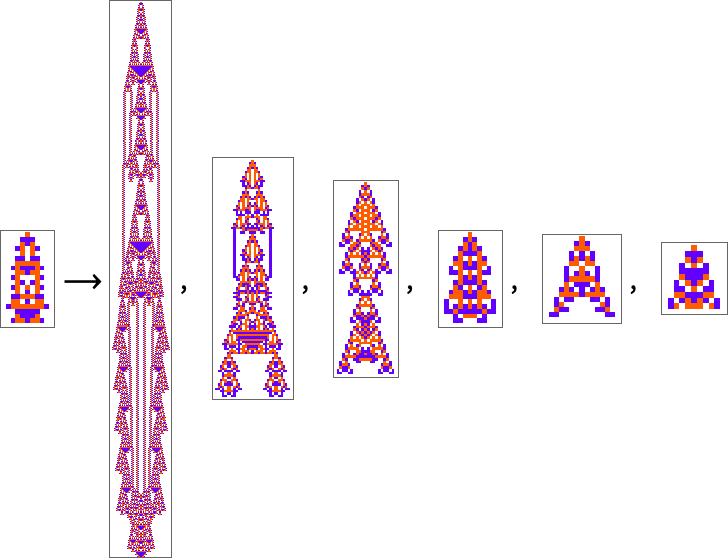
Starting from the null rule, the number of phenotypes reached after successively more (non-fitness-neutral) mutations is

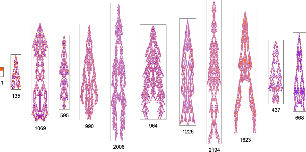
and the successive longest-lived of these phenotypes are:
Aspect Ratio Fitness
Just as we looked at fitness functions based on aspect ratio above for symmetric k = 2, r = 2 rules, so now we can do this for the whole space of all possible k = 2, r = 2 rules. Here’s a plot of the heights and widths of patterns that can be achieved with these rules:
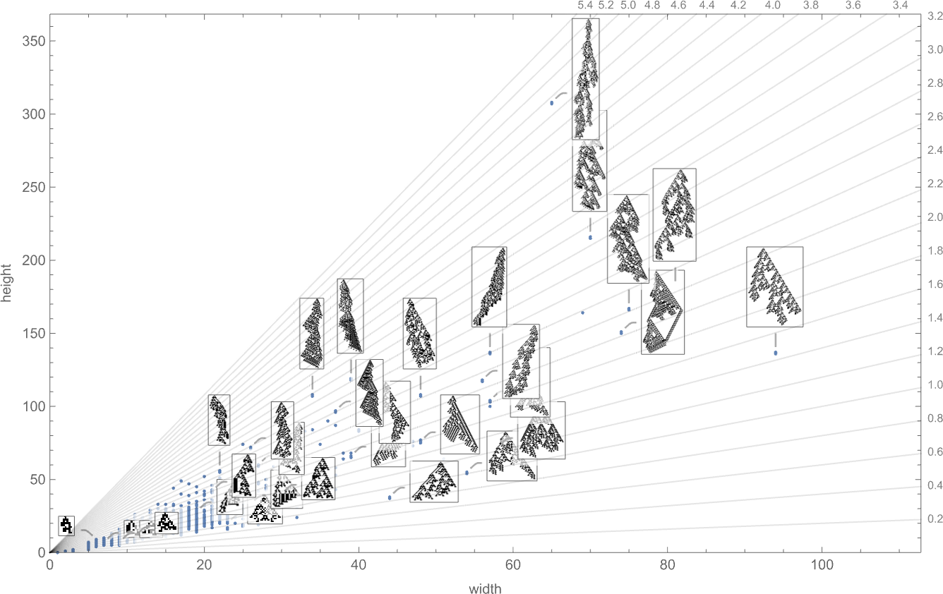
These are the possible aspect ratios this implies:

And here’s their distribution (on a log scale):

The range of possible values extends much further than for symmetric k = 2, r = 2 rules:  to
to  rather than
  to
to  . The patterns now with the largest aspect ratios are
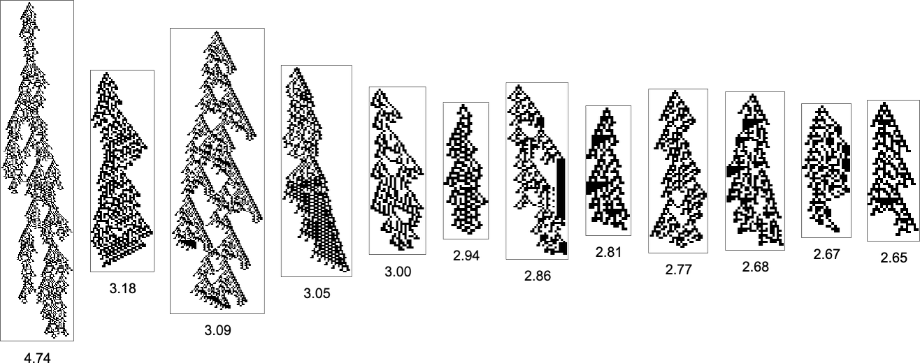
while those with the smallest aspect ratios are:

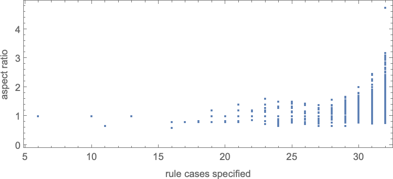
Note that just as for symmetric k = 2, r = 2 rules, to reach a wider range of aspect ratios, more cases in the rule have to be specified:
So what happens if we use adaptive evolution to try to reach different possible target aspect ratios? Most of the time (at least up to aspect ratio ≈ 3) there’s some sequence of mutations that will do it—though often we can get stuck at a different aspect ratio:

If we look at the “best convergence” to a given target aspect ratio then we see that this improves as we increase the number of cases specified in the rule:

So what does the multiway graph look like for a fitness function associated with a particular aspect ratio? Here’s the result for aspect ratio 3:
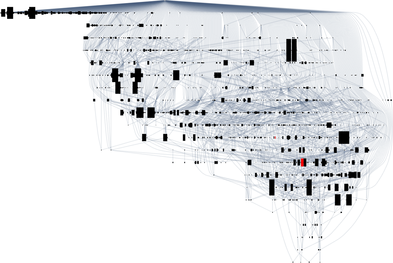
The initial node involves patterns with aspect ratio 1—actually a fitness-neutral set of 263 of them. And as we go through the multiway graph, the aspect ratios get nearer to 3. The very closest they get, though, are for the patterns (whose locations are indicated on the graph):
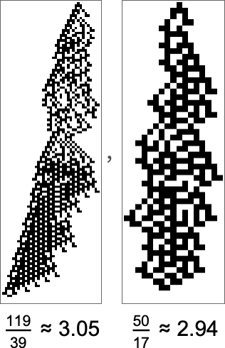
But actually (as we saw in the lineup above), there is a rule that gives aspect ratio exactly 3:
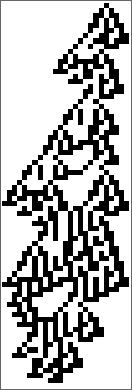
But it turns out that this rule can’t be reached by adaptive evolution using single point mutations. In effect, adaptive evolution isn’t “strong enough” to achieve the exact aspect ratio we want; we can think of it as being “unpredictably prevented” by computationally irreducible “developmental constraints”.
OK, so what about the symmetric k = 3, r = 1 rules? Here’s how they’re distributed in width and height:
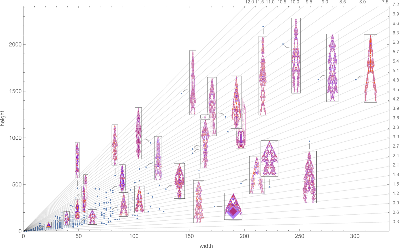
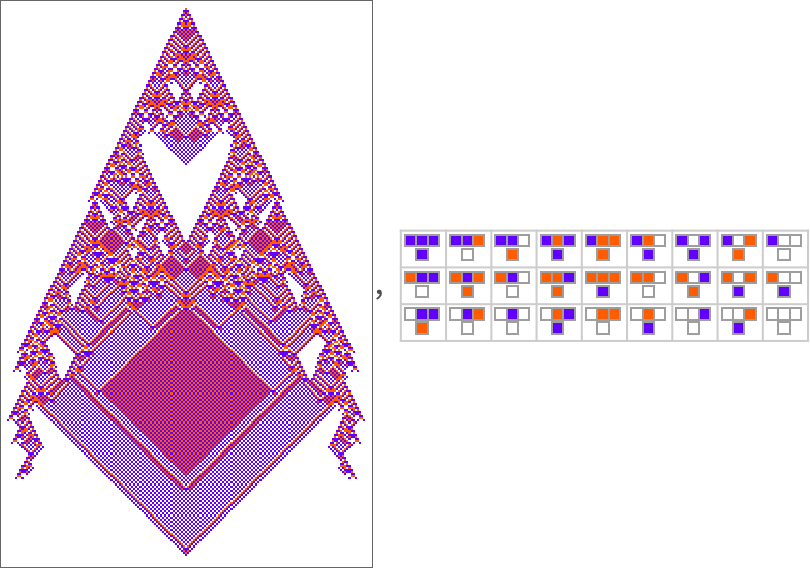
And, yes, in a typical “there are always surprises” story, there’s a strange height 265, width 173 pattern that shows up:
The overall possible aspect ratios are now

and their (log) distribution is:

The phenotypes with the largest aspect ratios are
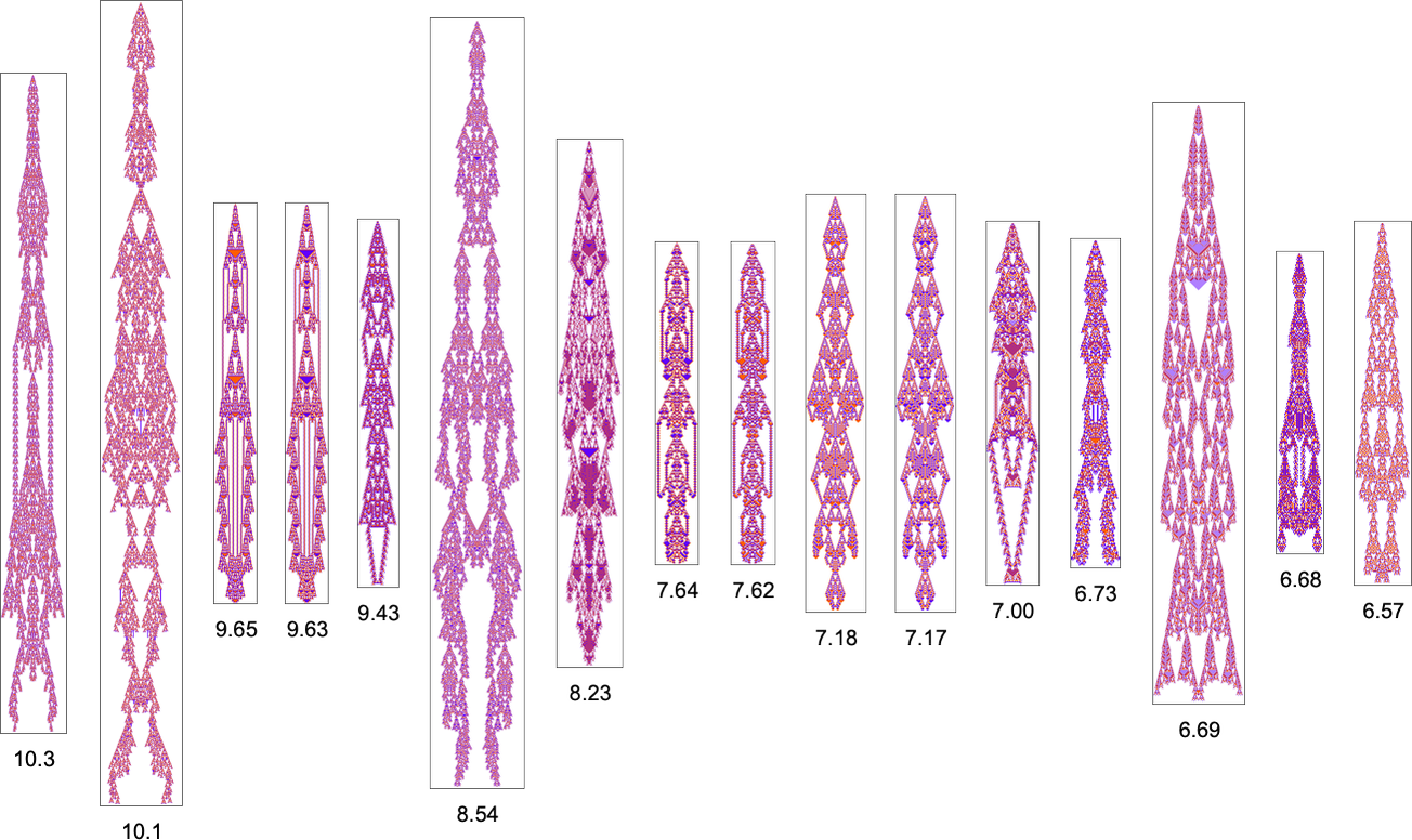
while those with the smallest aspect ratios are:

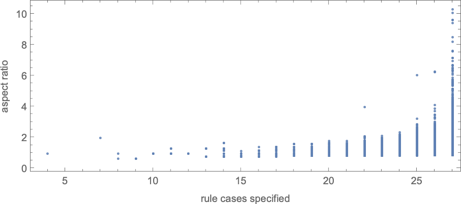
Once again, to reach a larger range of aspect ratios, one has to specify more cases in the rule:
If we try to target a certain aspect ratio, there’s somewhat more of a tendency to get stuck than for k = 2, r = 2 rules—perhaps somewhat as a result of there now being fewer total rules (though more phenotypes) available:

Branching in the Multiway Evolution Graph
Looking at a typical multiway evolution graph such as
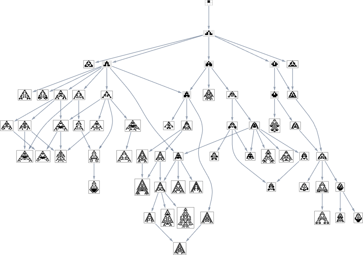
we see that different phenotypes can be quite separated in the graph—a bit like organisms on different branches of the tree of life in actual biology. But how can we characterize this separation? One approach is to compute the so-called dominator tree of the graph:
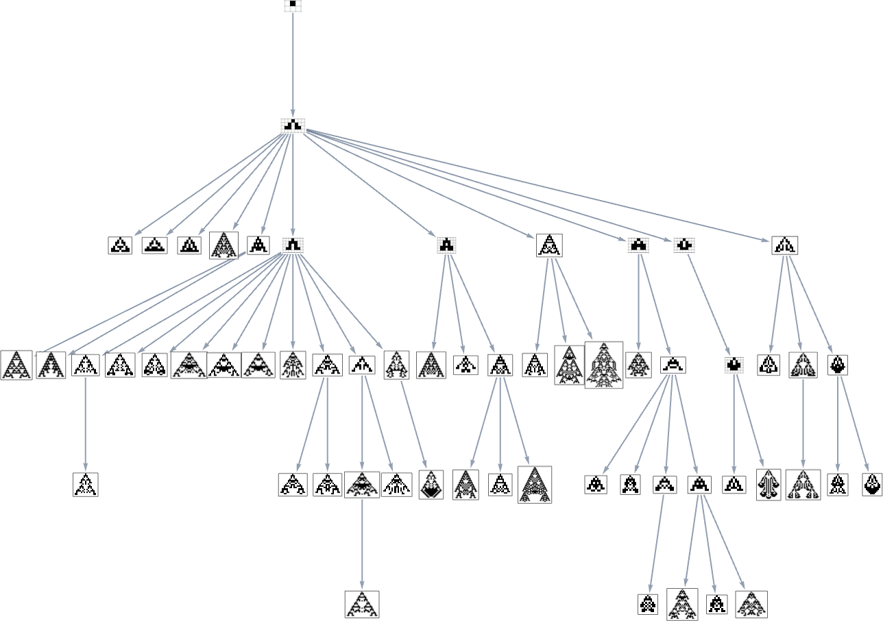
We can think of this as a way to provide a map of the least common ancestors of all nodes. The tree is set up so that given two nodes you just trace up the tree to find their common ancestor. Another interpretation of the tree is that it shows you what nodes you have no choice but to pass through in getting from the initial node to any given node—or, in other words, what phenotypes adaptive evolution has to produce on the way to a given phenotype.
Here’s another rendering of the tree:
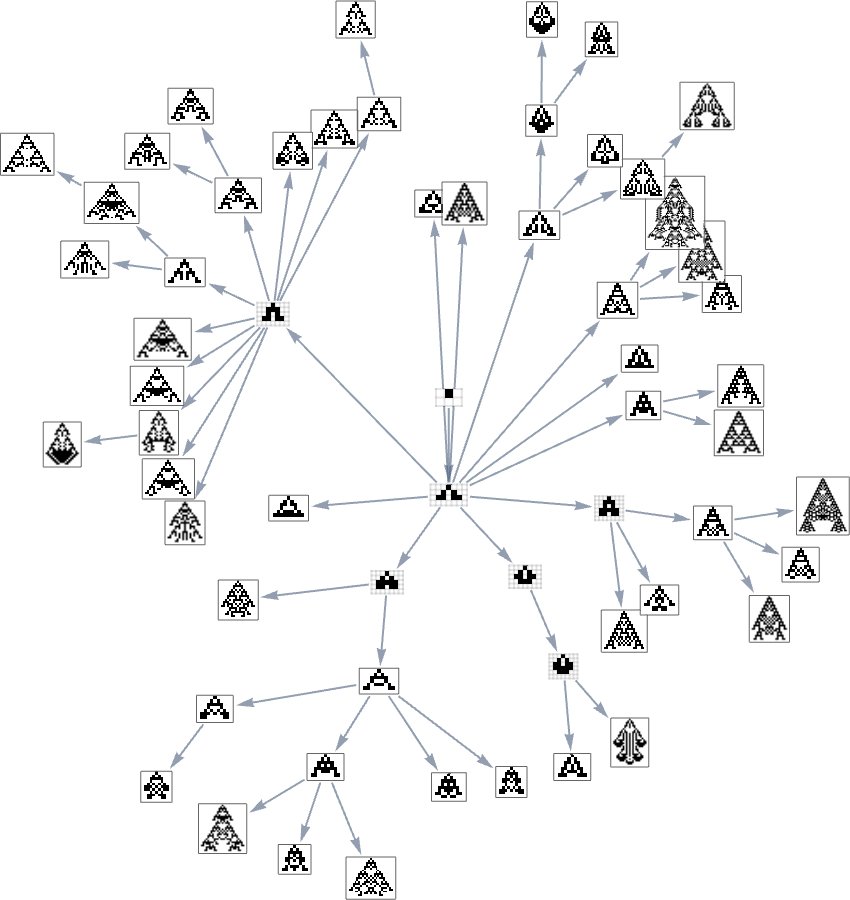
We can think of this as the analog of the biological tree of life, with successive branchings picking out finer and finer “taxonomic domains” (analogous to kingdoms, phyla, etc.)
The tree also shows us something else: how significant different links or nodes are—and how much of the tree one would “lop off” if they were removed. Or, put a different way, how much would be achieved by blocking a certain link or node—as one might imagine doing to try to block the evolution of bacteria or tumor cells?
What if we look at larger multiway evolution graphs, like the complete k = 2, r = 2 one? Once again we can construct a dominator tree:
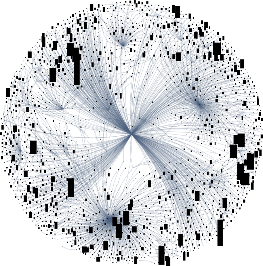
It’s notable that there’s tremendous variance in the “fan out” here, with the phenotypes with largest successor counts being the rather undistinguished:

But what if one’s specifically trying to reach, say, one of the maximum lifetime (length 308) phenotypes? Well, then one has to follow the paths in a particular subgraph of the original multiway evolution graph
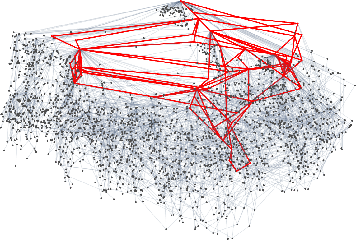
corresponding to the phenotype graph:
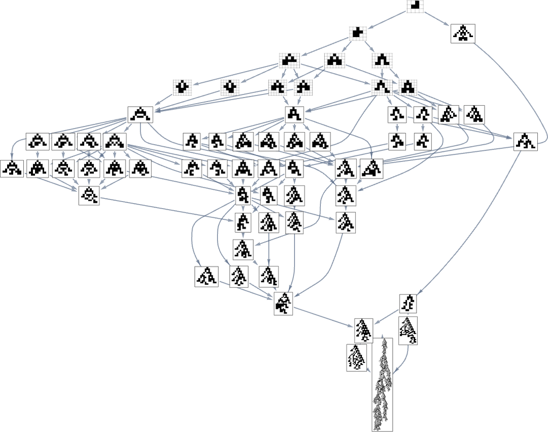
If one goes off this “narrow path” then one simply can’t reach the length-308 phenotype; one inevitably gets stuck in what amounts to another branch of the analog of the “tree of life”. So if one is trying to “guide evolution” to a particular outcome, this tells one that one needs to block off lots of “exit ramps”.
But what “fraction of the whole graph” is the subgraph that leads to the length-308 phenotype? The whole graph has 2409 vertices and 3878 edges, while the subgraph has 64 vertices and 119 edges, i.e. in both cases about 3%. A different measure is what fraction of all paths through the graph lead to the length-308 phenotype. The total number of paths is 606,081, while the number leading to the length-308 phenotype is 1260, or about 0.2%. Does this tell us what the probability of reaching that phenotype will be if we just make a random sequence of mutations? Not quite, because in the multiway evolution graph many equivalencings have been done, notably for fitness-neutral sets. And if we don’t do such equivalencings, it turns out (as we’ll discuss below) that the corresponding number is significantly smaller—about 0.007%.
Exact-Match Fitness Functions
The fitness functions we’ve been considering so far look only at coarse features of phenotype patterns—like their height, width and aspect ratio. But what happens if we have a fitness function that’s maximal only for a phenotype that exactly matches a particular pattern?
As an example, let’s consider k = 2, r = 1 cellular automata with phenotypes grown for a specific number of steps—and with a fitness function that counts the number of cells that agree with ones in a target:

Let’s say we start with the null rule, then adaptively evolve by making single point mutations to the rule (here just 8 bits). With a target of the rule 30 pattern, this is the multiway graph we get:
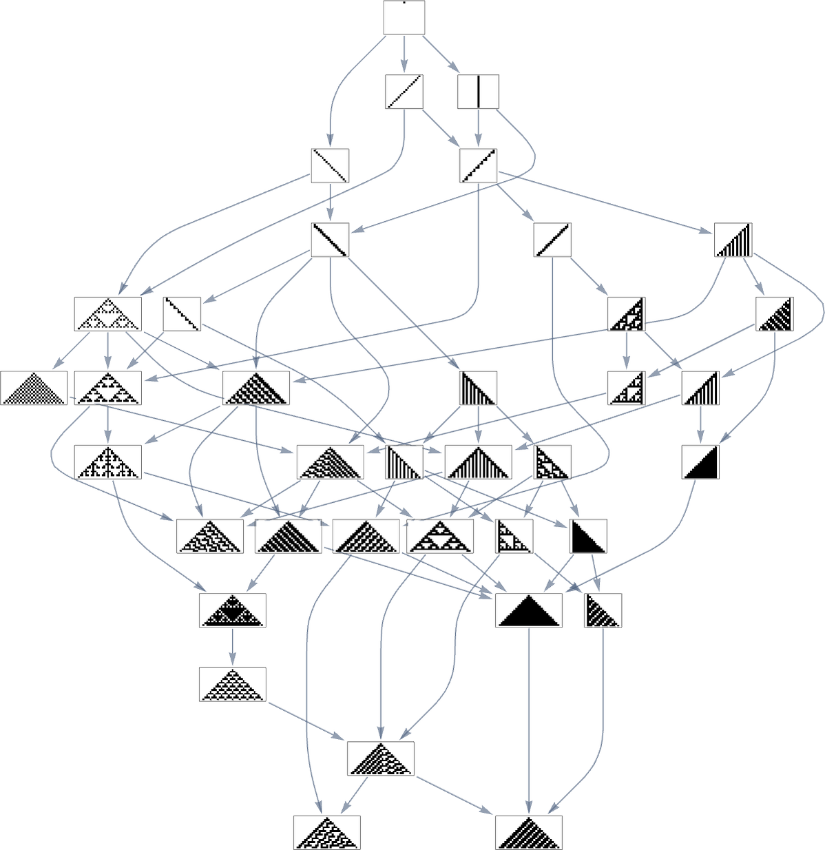
And what we see is that after a grand tour of nearly a third of all possible rules, we can successfully reach the rule 30 pattern. But we can also get stuck at rule 86 and rule 190 patterns—even though their fitness values are much lower:

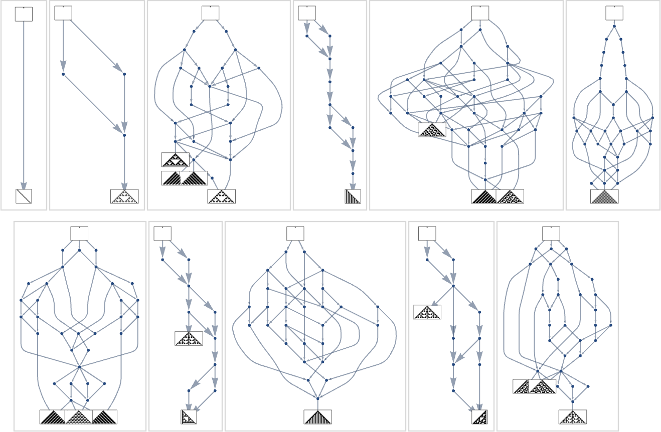
If we consider all possible k = 2, r = 1 cellular automaton patterns as targets, it turns out that these can always be reached by adaptive evolution from the null rule—though a little less than half the time there are other possible endpoints (here specified by rule numbers) at which the evolution process can get stuck:
So far we’ve been assuming that we have a fitness function that’s maximized by matching some pattern generated by a cellular automaton pattern. But what if we pick some quite different pattern to match against? Say our pattern is:
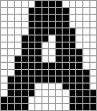
With k = 2, r = 1 rules (running with wraparound in a finite-size region), we can construct a multiway graph
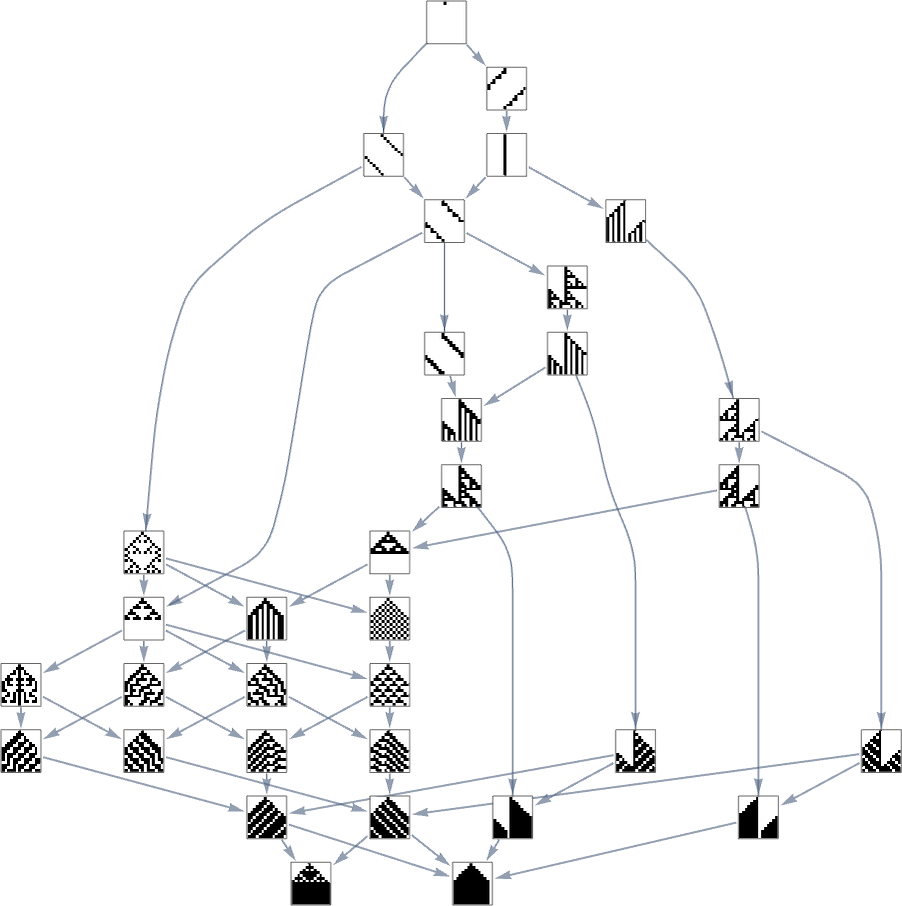
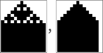
and find out that the maximum fitness endpoints are the not-very-good approximations:
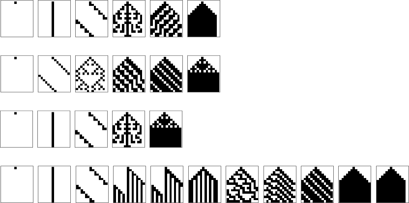
We can also get to these by applying random mutations:
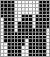
But what if we try a larger rule space, say k = 2, r = 2 rules? Our approximations to the “A” image get a bit better:
Going to k = 2, r = 3 leads to slightly better (but not great) final approximations:

If we try to do the same thing with our target instead being

we get for example

while with target
we get (even less convincing) results like:

What’s going on here? Basically it’s that if we try to set up too intricate a fitness function, then our rule spaces won’t contain rules that successfully maximize it, and our adaptive evolution process will end up with a variety of not-very-good approximations.
How Fitness Builds Up
When one looks at an evolution process like
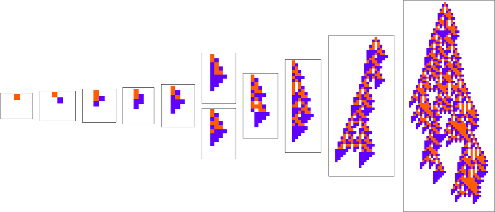
one typically has the impression that successive phenotypes are achieving greater fitness by somehow progressively “building on the ideas” of earlier ones. And to get a more granular sense of this we can highlight cells at each step that are using “newly added cases” in the rule:
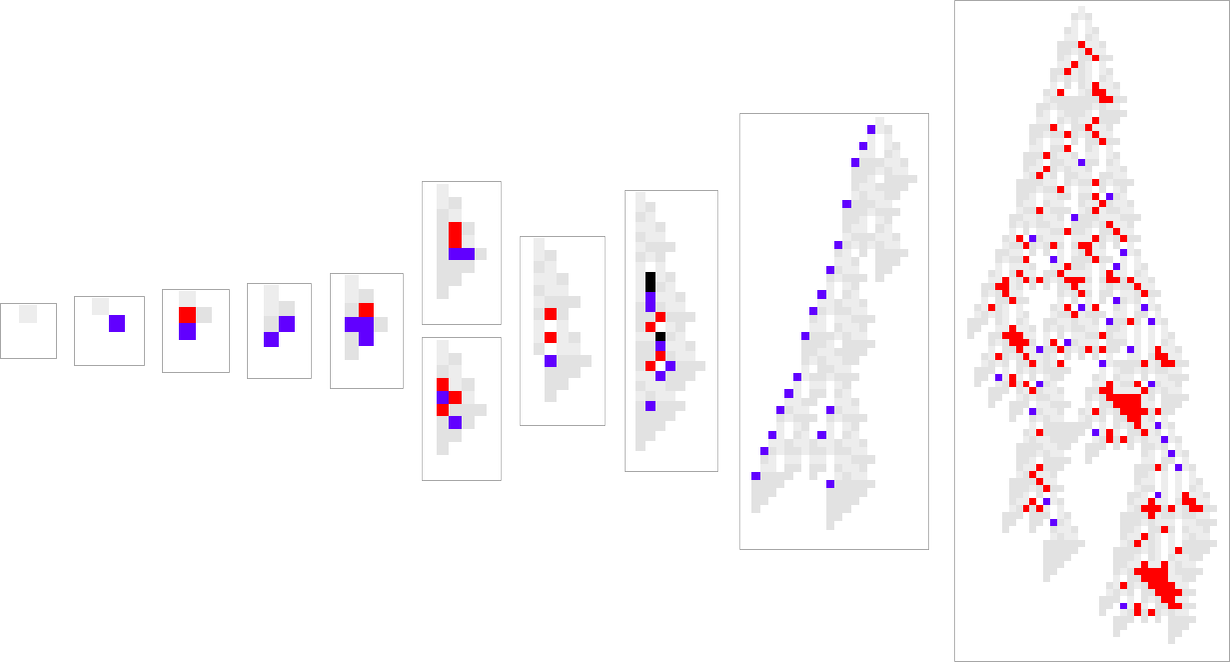
We can think of new rule cases as a bit like new genes in biology. So what we’re seeing here is the analog of new genes switching on (or coming into existence) as we progress through the process of biological evolution.
Here’s what happens for some other paths of evolution:
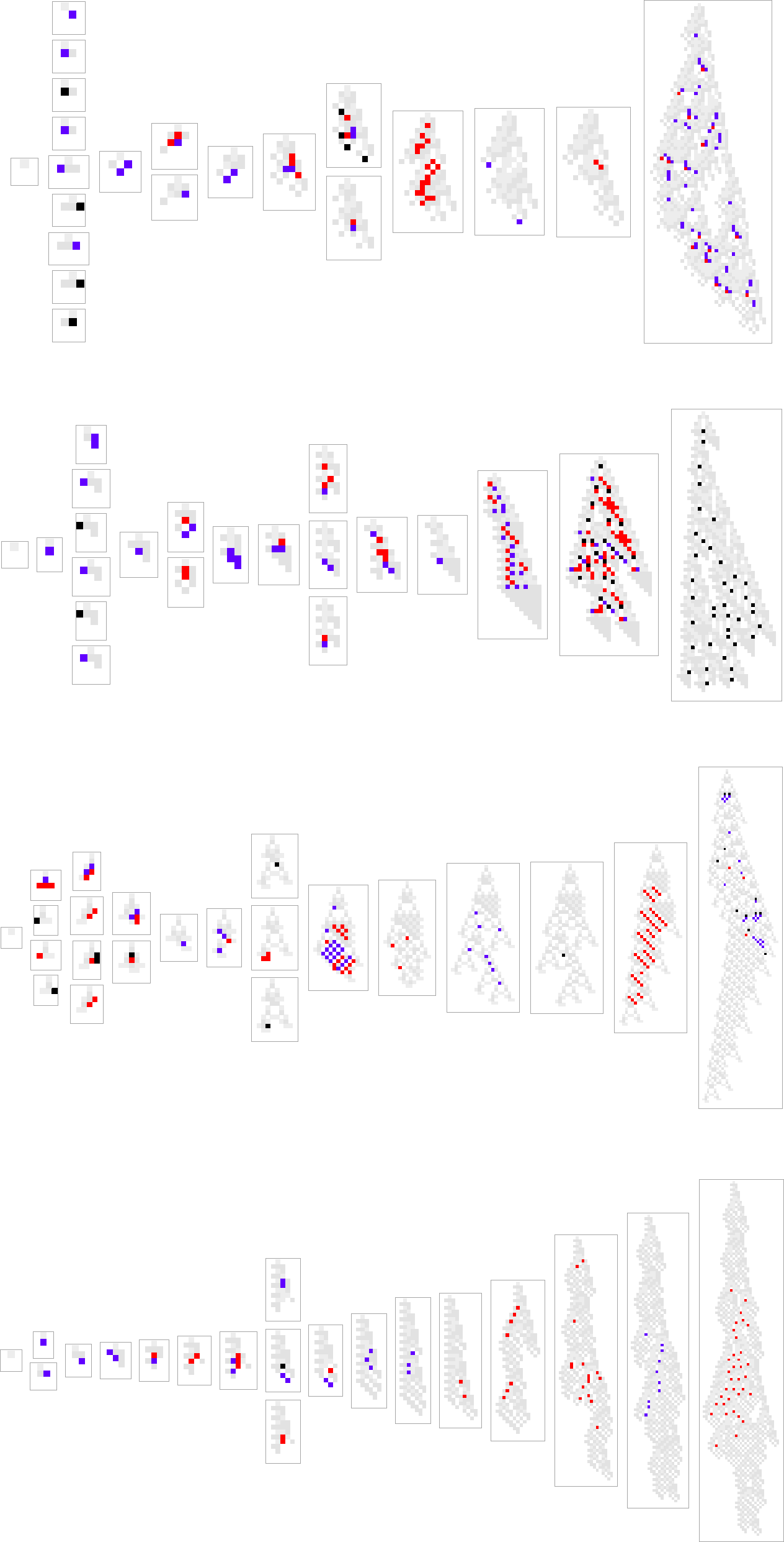
What we see is quite variable. There are a few examples where new rule cases show up only at the end, as if a new “incrementally engineered” pattern was being “grafted on at the end”. But most of the time new rule cases show up sparsely dotted all over the pattern. And somehow those few “tweaks” lead to higher fitness—even though there’s no obvious reason why, and no obvious way to predict where they should be.
It’s interesting to compare this with actual biology, where it’s pretty common to see what appear to be “random gratuitous changes” between apparently very similar organisms. (And, yes, this can lead to all sorts of problems in things like comparing toxicity or drug effectiveness in model animals versus humans.)
There are many ways to consider quantitatively characterizing how “rule utilization” builds up. As just one example, here are plots for successive phenotypes along the evolution paths shown above of what stages in growth new rule cases show up:


But Is It Explainable?
Here are two “adaptively evolved” long-lifetime rules that we discussed at the beginning:
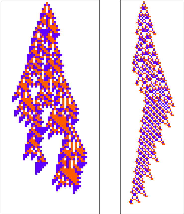
We can always run these rules and see what patterns they produce. But is there a way to explain what they do? And for example to analyze how they manage to yield lifetimes? Or is what we’re seeing in these rules basically “pure computational irreducibility” where the only way to tell what patterns they will generate—and how long they’ll live—is just explicitly to run them step by step?
The second rule here seems to have a bit more regularity than the first, so let’s tackle it first. Let’s look at the “blade” part. Once such an object—of any width—has formed, its behavior will basically be repetitive, and it’s easy to predict what will happen:
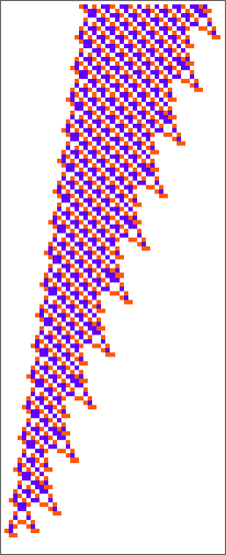
The left-hand edge moves by 1 position every 7 steps, and the right-hand edge by 4 positions every 12 steps. And since  , however wide the initial configuration is, it’ll always die out, after a number of steps that’s roughly
  times the initial width.
But OK, how does a configuration like this get produced? Well, that’s far from obvious. Here’s what happens with a sequence of few-cell initial conditions  …:
…:

So, yes, it doesn’t always directly make the “blade”. Sometimes, for example, it instead makes things like these, some of which basically just become repetitive, and live forever:
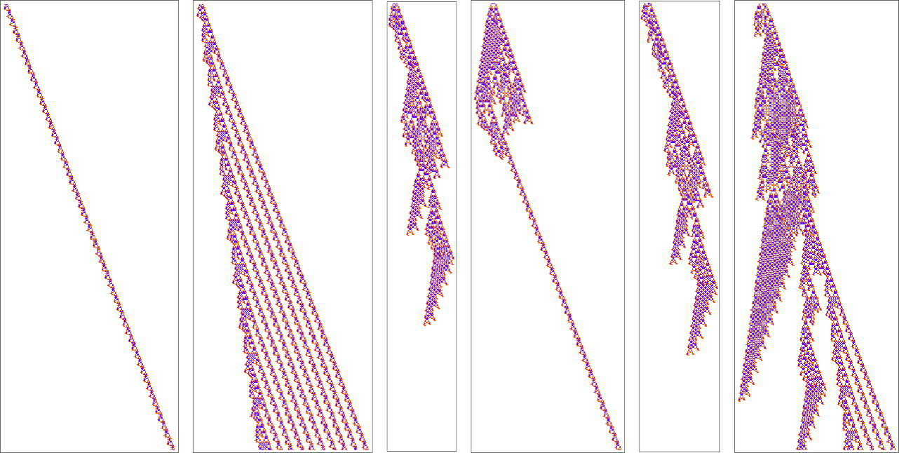
And even if it starts with a “blade texture” unexpected things can happen:

There are repetitive patterns that can persist—and indeed the “blade” uses one of these:

Starting from a random initial condition one sees various kinds of behavior, with the blade being fairly common:
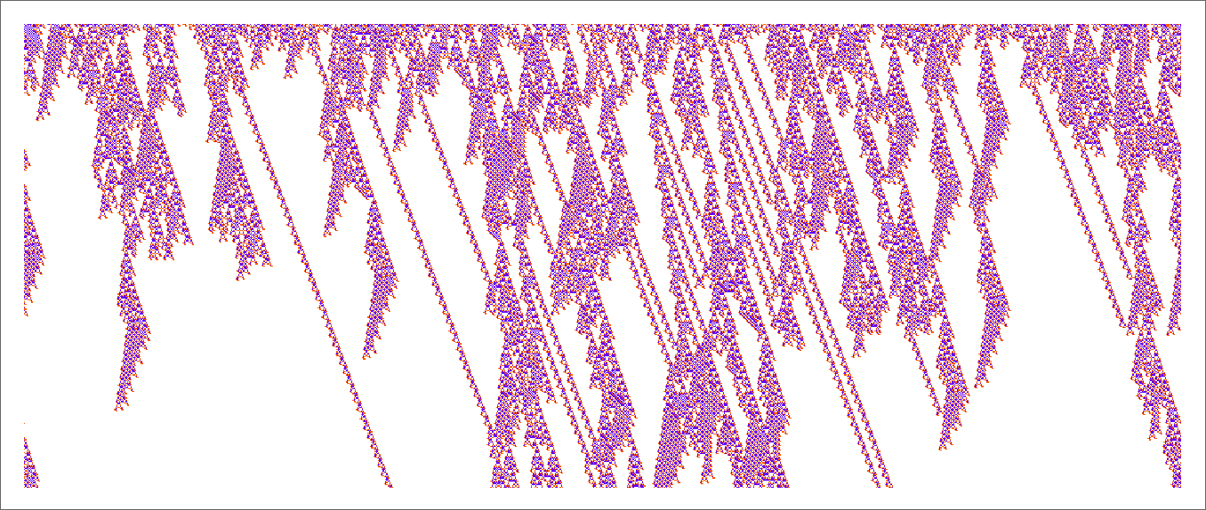
But none of this really makes much of a dent in “explaining” why with this rule, starting from a single red cell, we get a long-lived pattern. Yes, once the “blade” forms, we know it’ll take a while to come to a point. But beyond this little pocket of computational reducibility we can’t say much in general about what the rule does—or why, for example, a blade forms with this initial condition.
So what about our other rule? There’s no obvious interesting pocket of reducibility there at all. Looking at a sequence of few-cell initial conditions we get:

And, yes, there’s all sorts of different behavior that can occur:
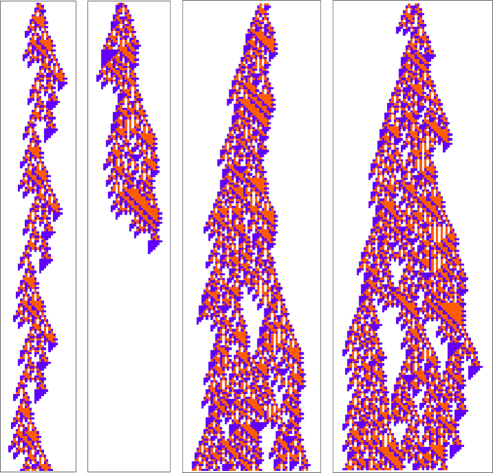
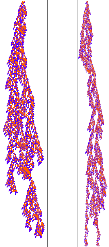
The first of these patterns is basically periodic, simply shifting 2 cells to the left every 56 steps. The third one dies out after 369 steps, and the fourth one becomes basically periodic (with period 56) after 1023 steps:
If we start from a random initial condition we see a few places where things die out in a repeatable pattern. But mostly everything just looks very complicated:
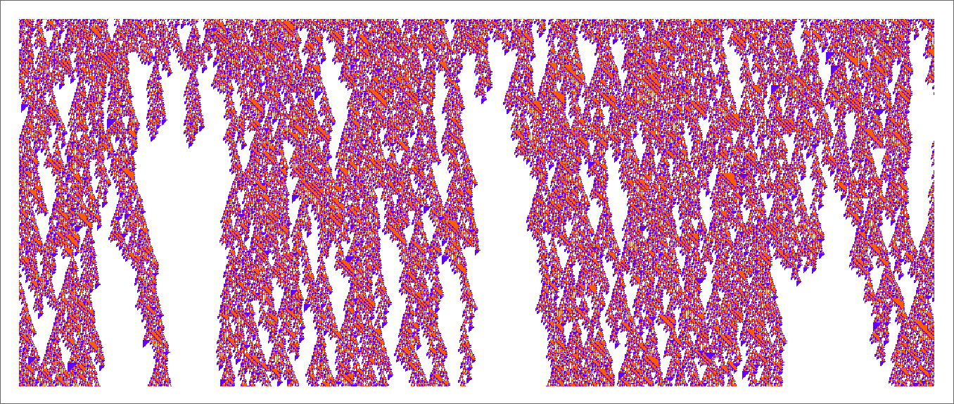
As always happens, the rule supports regions of repetitive behavior, but they don’t normally extend far enough to introduce any significant computational reducibility:

So what’s the conclusion? Basically it’s that these rules—like pretty much all others we’ve seen here—behave in essentially computationally irreducible ways. Why do they have long lifetimes? All we can really say is “because they do”. Yes, we can always run them and see what happens. But we can’t make any kind of “explanatory theory”, for example of the kind we’re used to in mathematical approaches to physics.
Distribution in Morphospace
We can think of the pattern of growth seen in each phenotype as defining what we might call in biology its “morphology”. So what happens if we try to operate as “pure taxonomists”, laying out different phenotypes in “morphospace”? Here’s a result based on using machine learning and FeatureSpacePlot:
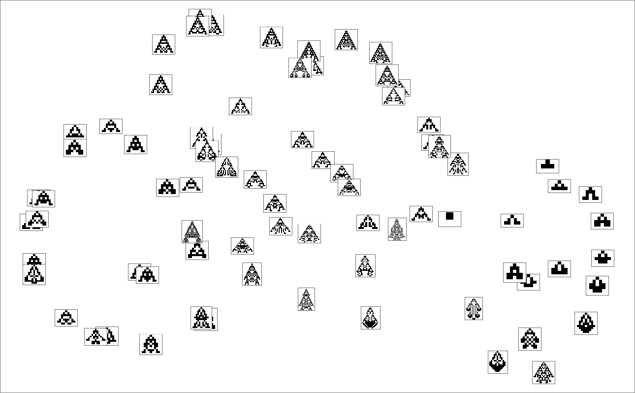
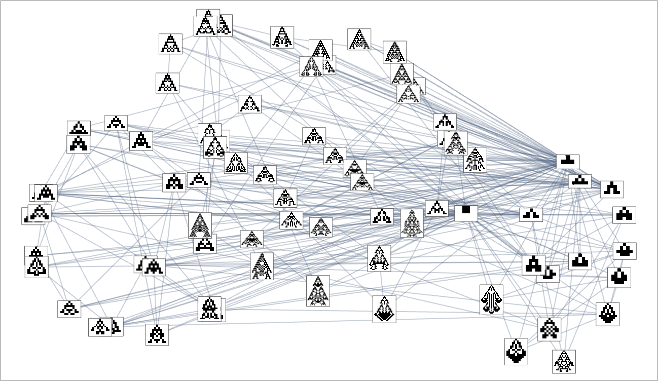
And, yes, this tends to group “visually similar” phenotypes together. But how does proximity in morphospace relate to proximity in genotypes? Here is the same arrangement of phenotypes as above, but now indicating the transformations associated with single mutations in genotype:
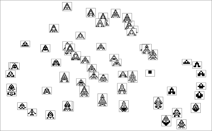
If for example we consider maximizing for height, only some of the phenotypes are picked out:
For width, a somewhat different set are picked out:
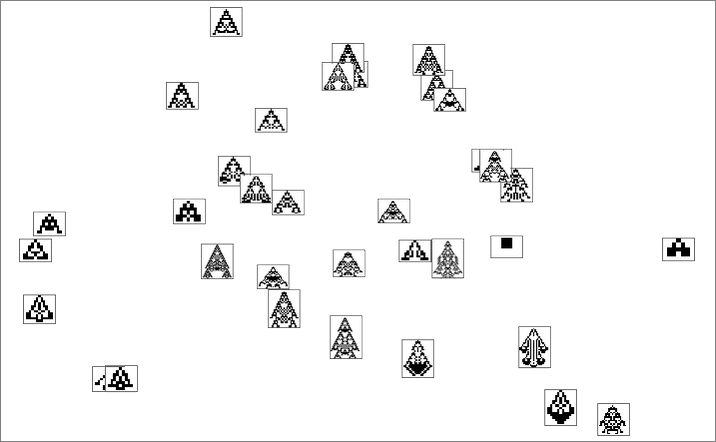
And here is what happens if our fitness function is based on aspect ratio:

In other words, different fitness functions “select out” different regions in morphospace.
We can also construct a morphospace not just for symmetric but for all k = 2, r = 2 rules:
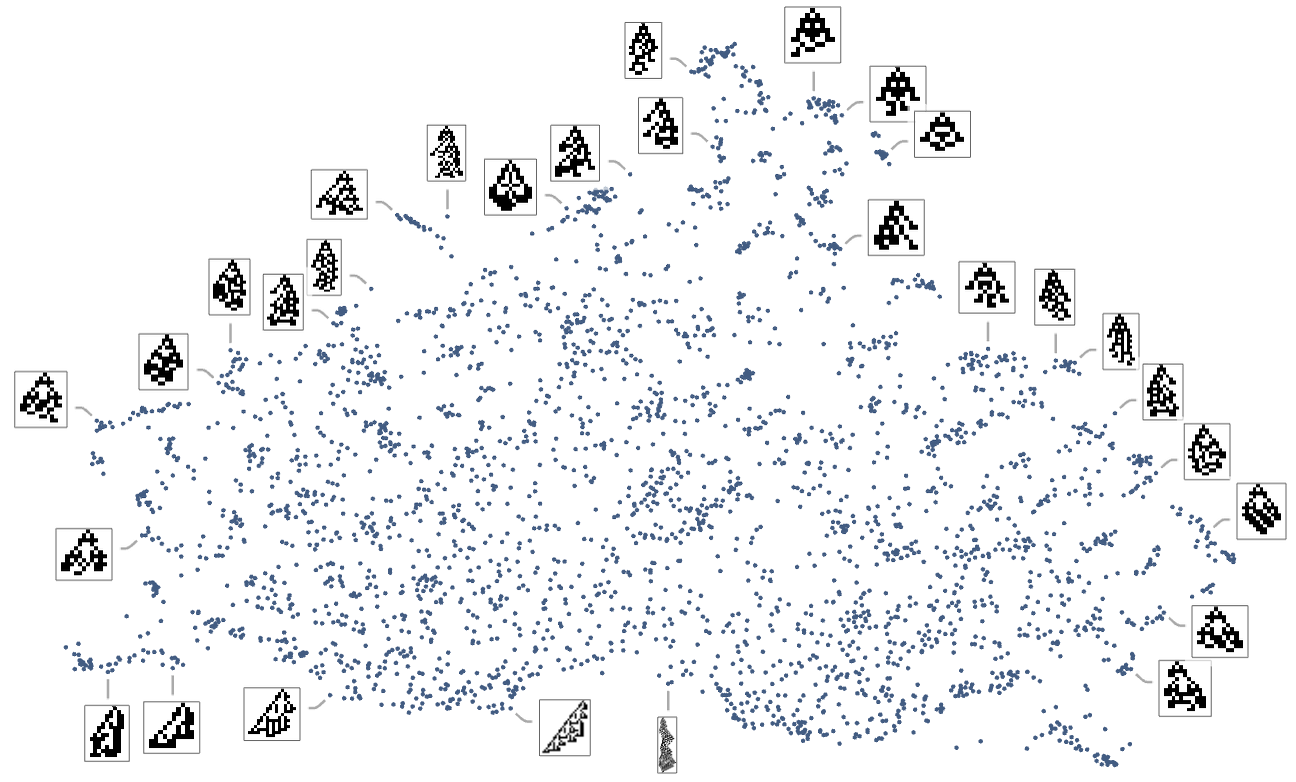
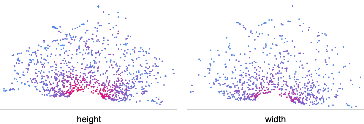
The detailed pattern here is not particularly significant, and, more than anything, just reflects the method of dimension reduction that we’ve used. What is more meaningful, however, is how different fitness functions select out different regions in morphospace. This shows the results for fitness functions based on height and on width—with points colored according to the actual values of height and width for those phenotypes:
Here are the corresponding results for fitness functions based on different aspect ratios, where now the coloring is based on closeness to the target aspect ratio:

What’s the main conclusion here? We might have expected that different fitness functions would cleanly select visibly different parts of morphospace. But at least with our machine-learning-based way of laying out morphospace that’s not what we’re seeing. And it seems likely that this is actually a general result—and that there is no layout procedure that can make any “easy to describe” fitness function “geometrically simple” in morphospace. And once again, this is presumably a consequence of underlying computational irreducibility—and to the fact that we can’t expect any morphospace layout procedure to be able to provide a way to “untangle the irreducibility” that will work for all fitness functions.
Probabilities and the Time Course of Evolution
In what we’ve done so far, we’ve mostly been concerned with things like what sequences of phenotypes can ever be produced by adaptive evolution. But in making analogies to actual biological evolution—and particularly to how it’s captured in the fossil record—it’s also relevant to discuss time, and to ask not only what phenotypes can be produced, but also when, and how frequently.
For example, let’s assume there’s a constant rate of point mutations in time. Then starting from a given rule (like the null rule) there’ll be a certain rate at which transitions to other rules occur. Some of these transitions will lead to rules that are selected out. Others will be kept, but will yield the same phenotype. And still others will lead to transitions to different phenotypes.
We can represent this by a “phenotype transition diagram” in which the thickness of each outgoing edge from a given phenotype indicates the fraction of all possible mutations that lead to the transition associated with that edge:
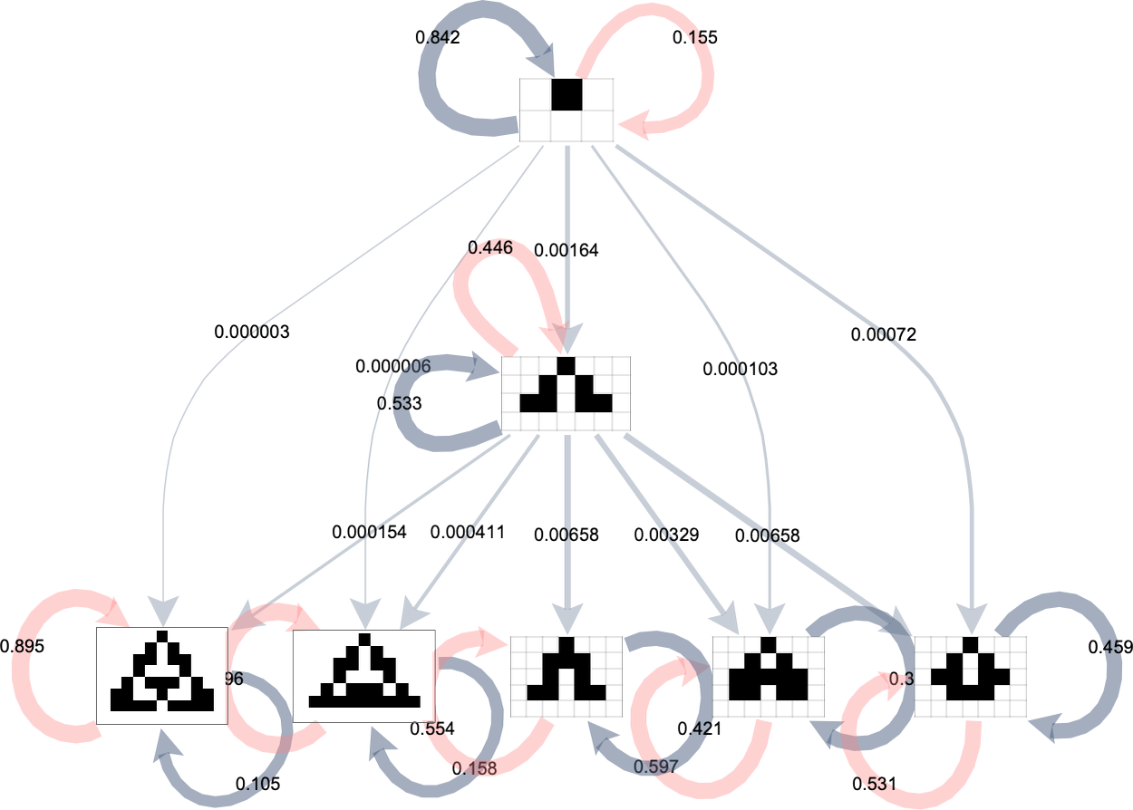
Gray self-loops in this diagram represent transitions that lead back to the same phenotype (because they change cases in the rule that don’t matter). Pink self-loops correspond to transitions that lead to rules that are selected out. We don’t show rules that have been selected out here; instead we assume that in this case we just “wait at the original phenotype” and don’t make a transition.
We can annotate the whole symmetric k = 2, r = 2 multiway evolution graph with transition probabilities:
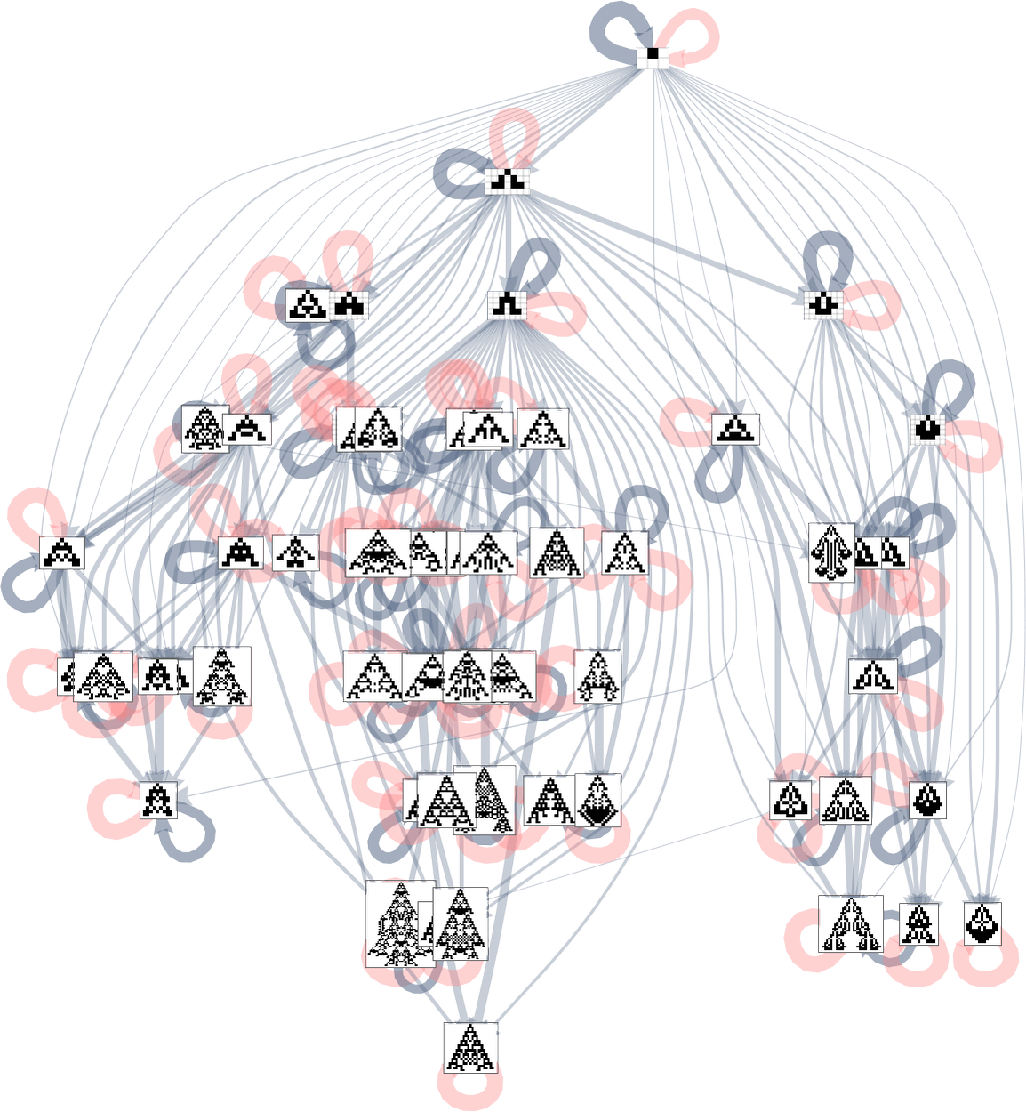
Underlying this graph is a matrix of transition probabilities between all 219 possible symmetric
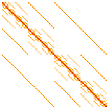
Keeping only distinct phenotypes and ordering by lifetime, we can then make a matrix of phenotype transition probabilities:
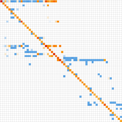
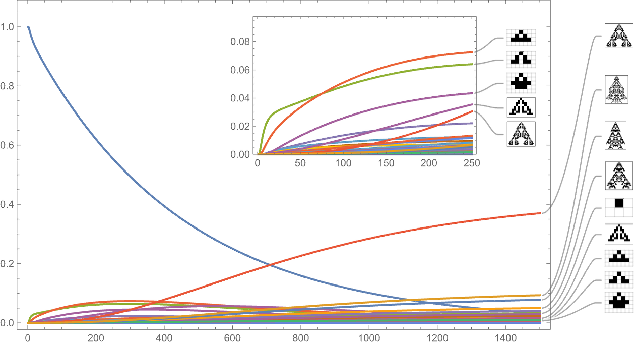
Treating the transitions as a Markov process, this allows us to compute the expected frequency of each phenotype as a function of time (i.e. number of mutations):
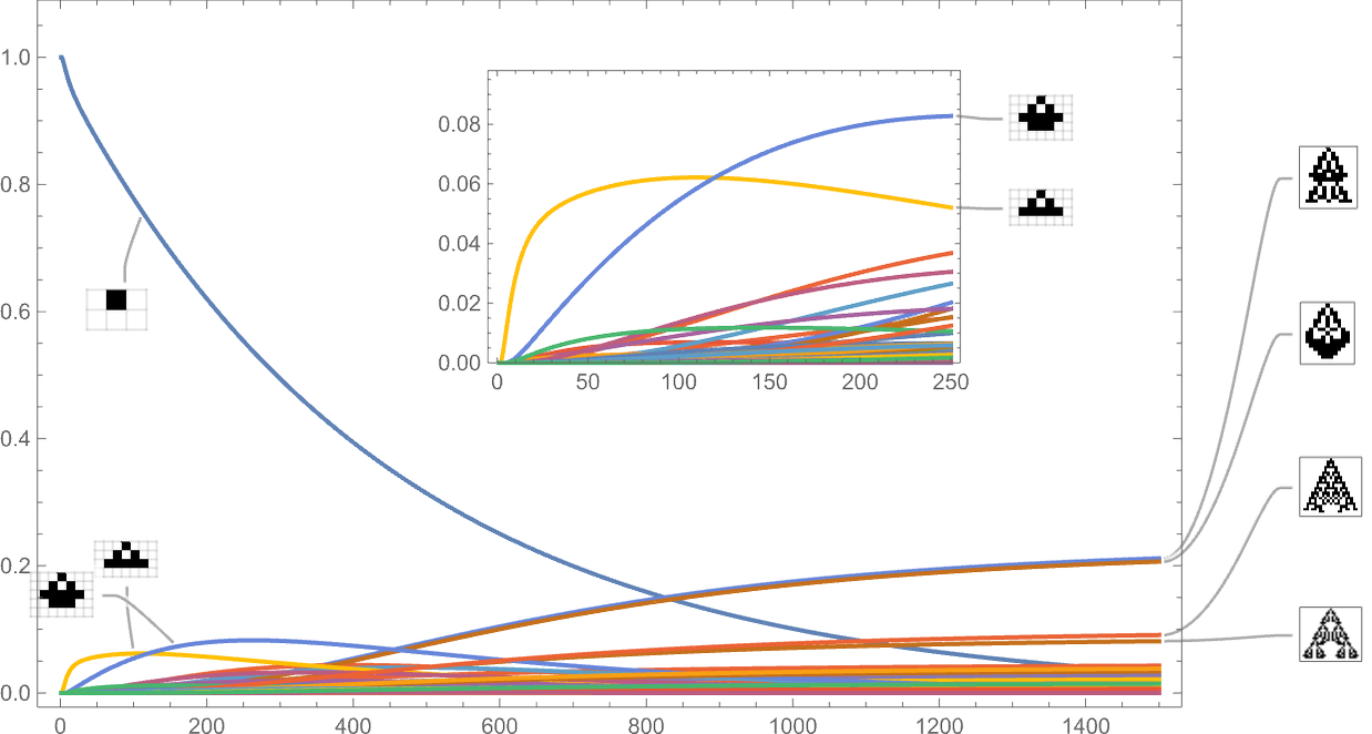
What’s basically happening here is that there’s steady evolution away from the single-cell phenotype. There are some intermediate phenotypes that come and go, but in the end, everything “flows” to the final (“leaf”) phenotypes on the multiway evolution graph—leading to a limiting “equilibrium” probability distribution:

Stacking the different curves, we get an alternative visualization of the evolution of phenotype frequencies:
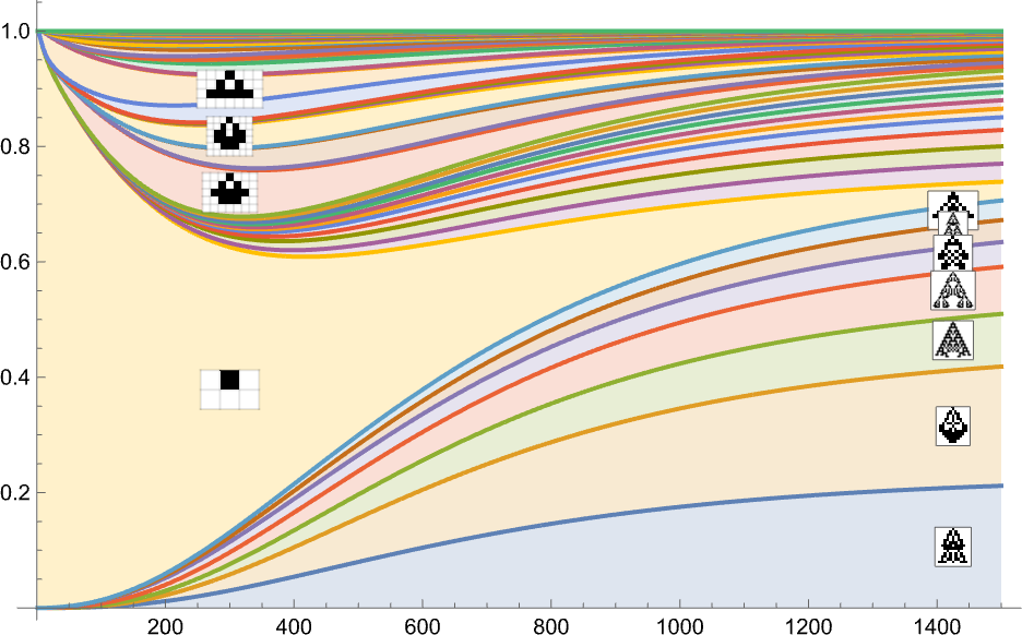
If we were “running evolution” with enough separate individuals, these would be the limiting curves we’d get. If we reduced the number of individuals, we’d start to see fluctuations—and there’d be a certain probability, for example, for a particular phenotype to end up with zero individuals, and effectively go extinct.
So what happens with a different fitness function? Here’s the result using width instead of height:
And here are results for fitness functions based on a sequence of targets for aspect ratio:
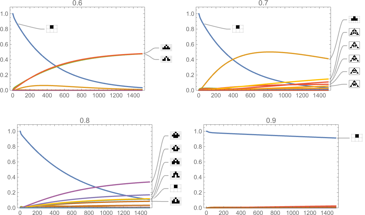
And, yes, the fitness function definitely influences the time course of our adaptive evolution process.
So far we’ve been looking only at symmetric k = 2, r = 2 rules. If we look at the space of all possible k = 2, r = 2 rules, the behavior we see is similar. For example, here’s the time evolution of possible phenotypes based on our standard height fitness function:
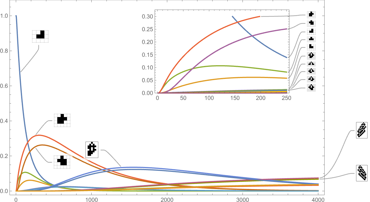
And this is what we see if we look only at the longest-lifetime (i.e. largest-height) cases:
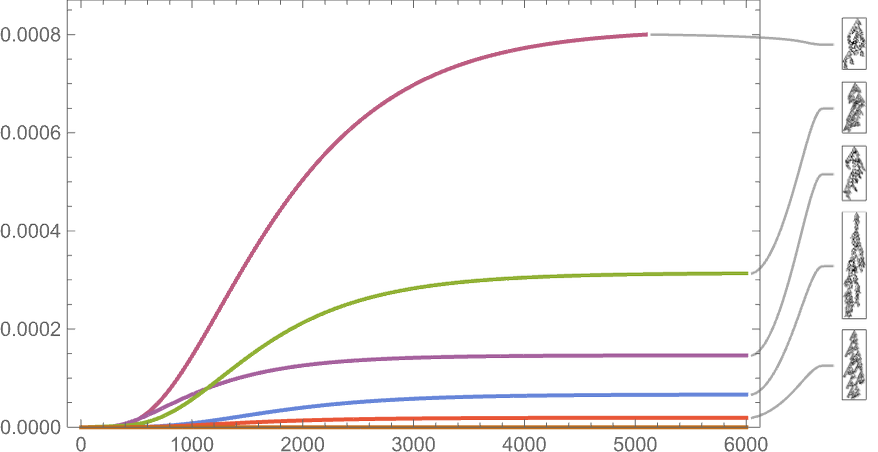
As the scale here indicates, such long-lived phenotypes are quite rare—though most still occur with nonzero frequency even after arbitrarily large times (which is an inevitable given that they appear as “maximal fitness” terminal nodes in the multiway graph).
And indeed if we plot the final frequencies of phenotypes against their lifetimes we see that there are a wide range of different cases:
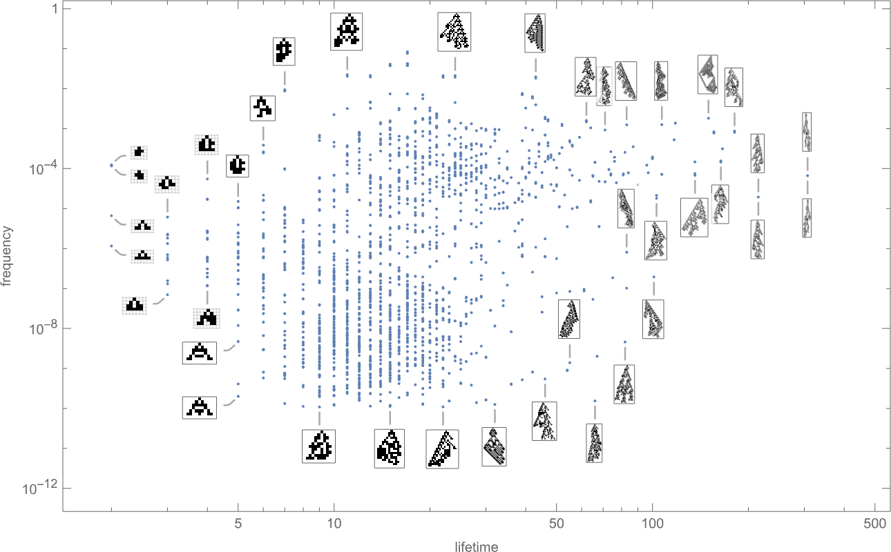
The phenotypes with the highest “equilibrium” frequencies are

with some having fairly small lifetimes, and others larger.
The Macroscopic Flow of Evolution
In the previous section, we looked at the time course of evolution with various different—but fixed—fitness functions. But what if we had a fitness function that changes with time—say analogous to an environment for biological evolution that changes with time?
Here’s what happens if we have an aspect ratio fitness function whose target value increases linearly with time:
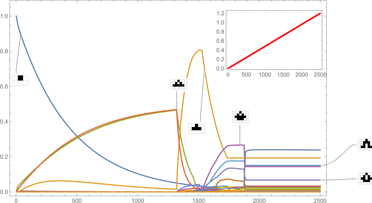
The behavior we see is quite complex, with certain phenotypes “winning for a while” but then dying out, often quite precipitously—with others coming to take their place.
If instead the target aspect ratio decreases with time, we see rather different behavior:
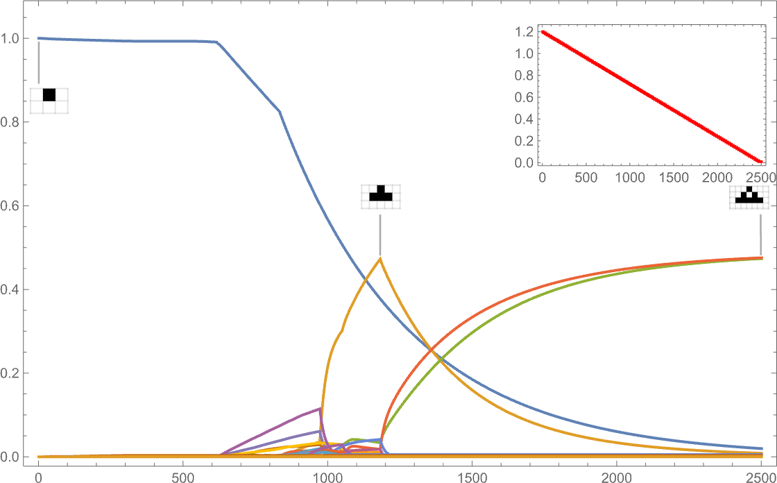
(The discontinuous derivatives here are basically associated with the sudden appearance of new phenotypes at particular target aspect ratio values.)
It’s also possible to give a “shock to the system” by suddenly changing the target aspect ratio:


And what we see is that sometimes this shock leads to fewer surviving phenotypes, and sometimes to more.
We can think of a changing fitness function as being something that applies a “macroscopic driving force” to our system. Things happen quickly down at the level of individual mutation and selection events—but the fitness function defines overall “goals” for the system that in effect change only slowly. (It’s a bit like a fluid where there are fast molecular-scale processes, but typically slow changes of macroscopic parameters like pressure.)
But if the fitness function defines a goal, how well does the system manage to meet it? Here’s a comparison between an aspect ratio goal (here, linearly increasing) and the distribution of actual aspect ratios achieved, with the darker curve indicating the mean aspect ratio obtained by a weighted average over phenotypes, and the lighter blue area indicating the standard deviation:
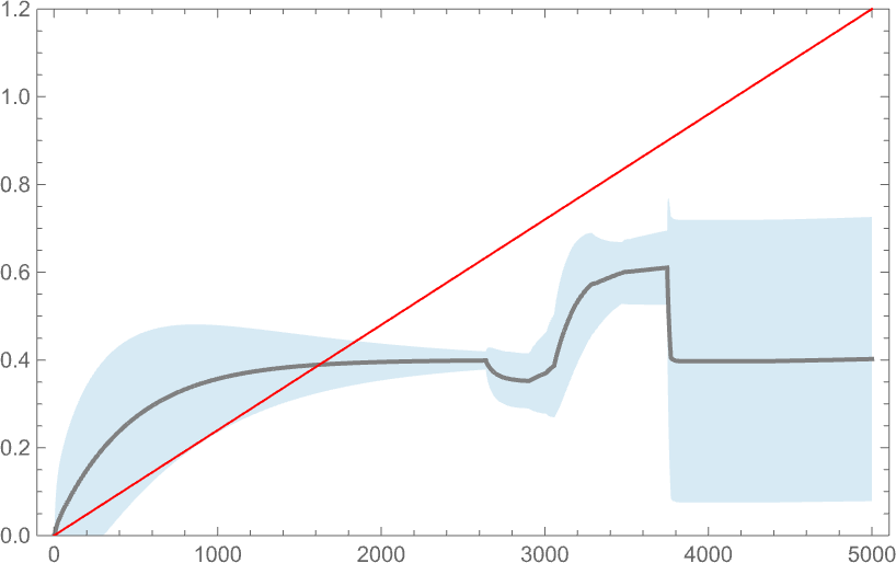
And, yes, as we might have expected from earlier results, the system doesn’t do particularly well at achieving the goal. Its behavior is ultimately not “well sculpted” by the forces of a fitness function; instead it is mostly dominated by the intrinsic (computationally irreducible) dynamics of the underlying adaptive evolution process.
One important thing to note however is that our results depend on the value of a parameter: essentially the rate at which underlying mutations occur relative to the rate of change of the fitness function. In the picture above 5000 mutations occur over the time the fitness function goes from minimum to maximum value. This is what happens if we change the number of mutations that occur (or, in effect, the “mutation rate”):

Generally—and not surprisingly—adaptive evolution does better at achieving the target when the mutation rate is higher, though in both the cases shown here, nothing gets terribly close to the target.
In their general character our results here seem reminiscent of what one might expect in typical studies of continuum systems, say based on differential equations. And indeed one can imagine that there might be “continuum equations of adaptive evolution” that govern situations like the ones we’ve seen here. But it’s important to understand that it’s far from self evident that this is possible. Because underneath everything is a multiway evolution graph with a definite and complicated structure. And one might think that the details of this structure would matter to the overall “continuum evolution process”. And indeed sometimes they will.
But—as we have seen throughout our Physics Project—underlying computational irreducibility leads to a certain inevitable simplicity when looking at phenomena perceived by computationally bounded observers. And we can expect that something similar can happen with biological evolution (and indeed adaptive evolution in general). Assuming that our fitness functions (and their process of change) are computationally bounded, then we can expect that their “aggregate effects” will follow comparatively simple laws—which we can perhaps think of as laws for the “flow of evolution” in response to external input.
Can Evolution Be Reversed?
In the previous section we saw that with different fitness functions, different time series of phenotypes appear, with some phenotypes, for example, sometimes “going extinct”. But let’s say evolution has proceeded to a certain point with a particular fitness function—and certain phenotypes are now present. Then one question we can ask is whether it’s possible to “reverse” that evolution, and revert to phenotypes that were present before. In other words, if we change the fitness function, can we make evolution “go backwards”?
We’ve often discussed a fitness function based on maximizing total (finite) lifetime. But what if, after using this fitness function for a while, we “reverse it”, now minimizing total lifetime?
Consider the multiway evolution graph for symmetric k = 2, r = 2 rules starting from the null rule, with the fitness function yet again being maximizing lifetime:
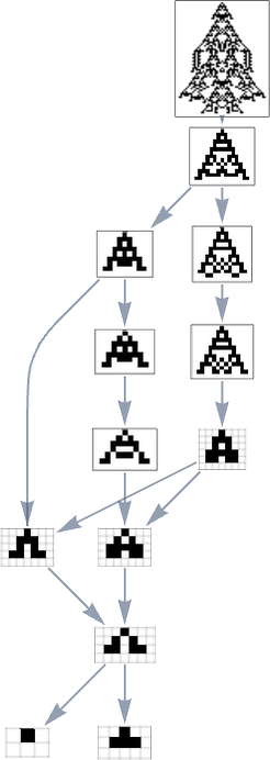
But what if we now say the fitness function minimizes lifetime? If we start from the longest-lifetime phenotype we get the “lifetime minimization” multiway graph:
We can compare this “reversed graph” to the “forward graph” based on all paths from the null rule to the maximum-lifetime rule:
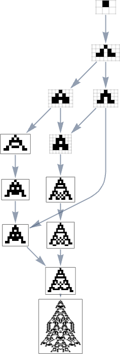
And in this case we see that the phenotypes that occur are almost the same, with the exception of the fact that  can appear in the reverse case.
So what happens when we look at all k = 2, r = 2 rules? Here’s the “reverse graph” starting from the longest-lifetime phenotype:
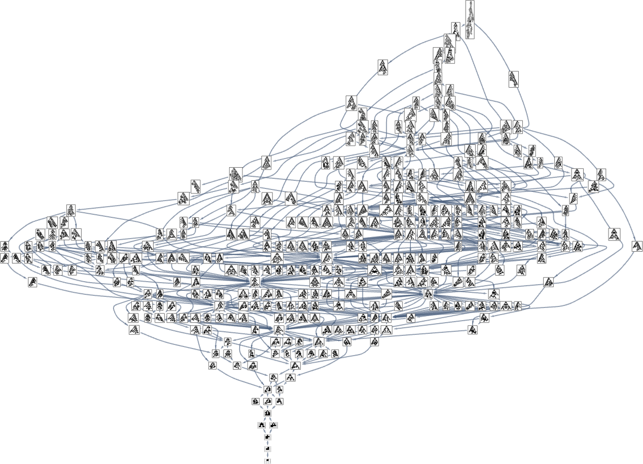
A total of 345 phenotypes appear here eventually leading all the way back to  . In the overall “forward graph” (which has to start from
  rather than
  ) a total of 2409 phenotypes appear, though (as we saw above) only 64 occur in paths that eventually lead to the maximum lifetime phenotype:
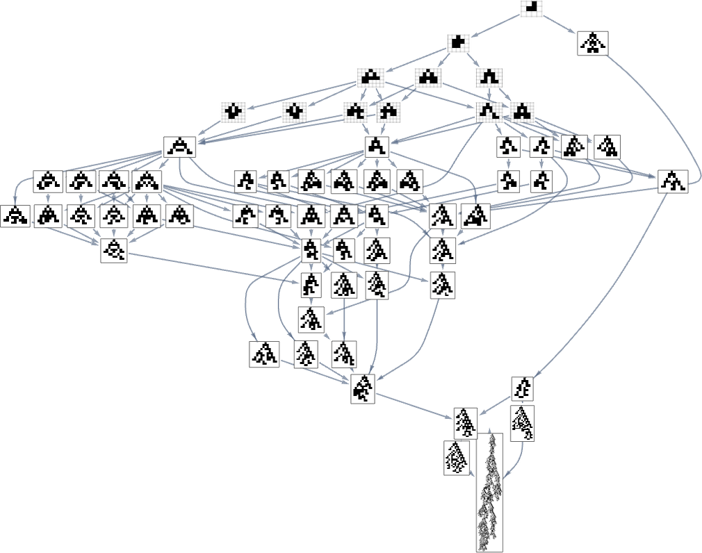
And what we see here is that the forward and reverse graphs look quite different. But could we perhaps construct a fitness function for the reverse graph that will successfully corral the evolution process to precisely retrace the steps of the forward graph?
In general, this isn’t something we can expect to be able to do. Because to do so would in effect require “breaking the computational irreducibility” of the system. It would require having a fitness function that can in essence predict every detail of the evolution process—and in so doing be in a position to direct it. But to achieve this, the fitness function would in a sense have to be computationally as sophisticated as the evolution process itself.
It’s a variant of an argument we’ve used several times here. Realistic fitness functions are computationally bounded (and in practice often very coarse). And that means that they can’t expect to match the computational irreducibility of the underlying evolution process.
There’s an analogy to the Second Law of thermodynamics. Just as the microscopic collisions of individual molecules are in principle easy to reverse, so potentially are individual transitions in the evolution graph. But putting many collisions or many transitions together leads to a process that is computationally sophisticated enough that the fairly coarse means at our disposal can’t “decode” and reverse it.
Put another way, there is in practice a certain inevitable irreversibility to both molecular dynamics and biological evolution. Yes, with enough computational effort—say carefully controlling the fitness function for every individual organism—it might in principle be possible to precisely “reverse evolution”. But in practice the kinds of fitness functions that exist in nature—or that one can readily set up in a lab—are computationally much too weak. And as a result one can’t expect to be able to get evolution to precisely retrace its steps.
Random or Selected? Can One Tell?
Given only a genotype, is there a way to tell whether it’s “just random” or whether it’s actually the result of some long and elaborate process of adaptive evolution? From the genotype one can in principle use the rules it defines to “grow” the corresponding phenotype—and then look at whether it has an “unusually large” fitness. But the question is whether it’s possible to tell anything directly from the genotype, without going through the computational effort of generating the phenotype.
At some level it’s like asking, whether, say, from a cellular automaton rule, one can predict the ultimate behavior of the cellular automaton. And a core consequence of computational irreducibility is that one can’t in general expect to do this. Still, one might imagine that one could at least make a “reasonable guess” about whether a genotype is “likely” to have been chosen “purely randomly” or to have been “carefully selected”.
To explore this, we can look at the genotypes for symmetric k = 2, r = 2 rules, say ordered by their lifetime-based fitness—with black and white here representing “required” rule cases, and gray representing undetermined ones (which can all independently be either black or white):
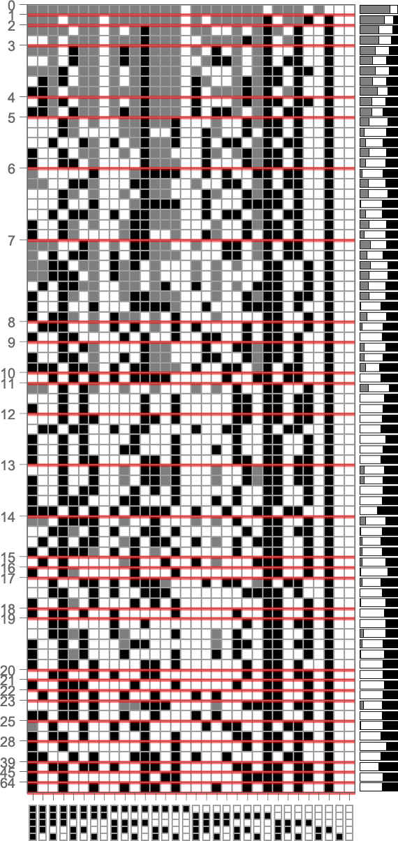
On the right is a summary of how many white, black and undetermined (gray) outcomes are present in each genotype. And as we have seen several times, to achieve high fitness all or almost all of the outcomes must be determined—so that in a sense all or almost all of the genome is “being used”. But we still need to ask whether, given a certain actual pattern of outcomes, we can successfully guess whether or not a genotype is the result of selection.
To get more of a sense of this, we can look at plots of the probabilities for different outcomes for each case in the rule, first (trivially) for all combinatorially possible genotypes, then for all genotypes that give viable (i.e. in our case, finite-lifetime) phenotypes, and then for “selected genotypes”:
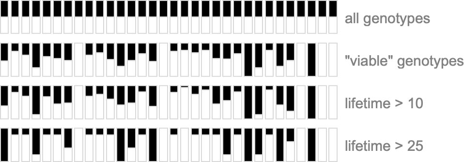
Certain cases are always completely determined for all viable genomes—but rather trivially so, because, for example, if  then the pattern generated will expand at maximum speed forever, and so cannot have a finite lifetime.
So what happens for all k = 2, r = 2 rules? Here are the actual genomes that lead to particular fitness levels:
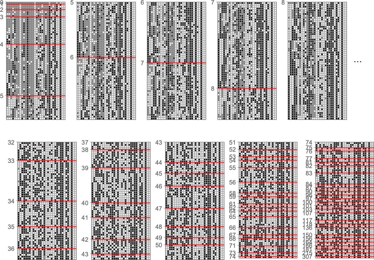
And now here are the corresponding probabilities for different outcomes for each case in the rule:
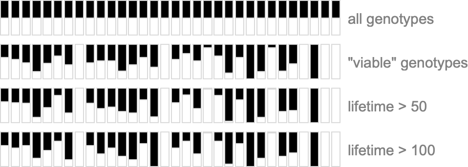
And, yes, given a particular setup we could imagine working out from results like these at least an approximation to the likelihood for a given randomly chosen genome to be a selected one. But what’s true in general? Is there something that can be determined with bounded computational effort (i.e. without explicitly computing phenotypes and their fitnesses) that gives a good estimate of whether a genome is selected? There are good reasons to believe that computational irreducibility will make this impossible.
It’s a different story, of course, if one’s given a “fully computed” phenotype. But at the genome level—without that computation—it seems unlikely that one can expect to distinguish random from “selected-somehow” genotypes.
Adaptive Evolution of Initial Conditions
In making our idealized model of biological evolution we’ve focused (as biology seems to) on the adaptive evolution of the genotype—or, in our case, the underlying rule for our cellular automata. But what if instead of changing the underlying rule, we change the initial condition used to “grow each organism”?
For example, let’s say that we start with the “single cell” we’ve been using so far, but then at each step in adaptive evolution we change the value of one cell in the initial condition (say within a certain distance of our original cell)—then keep any initial condition that does not lead to a shorter lifetime:
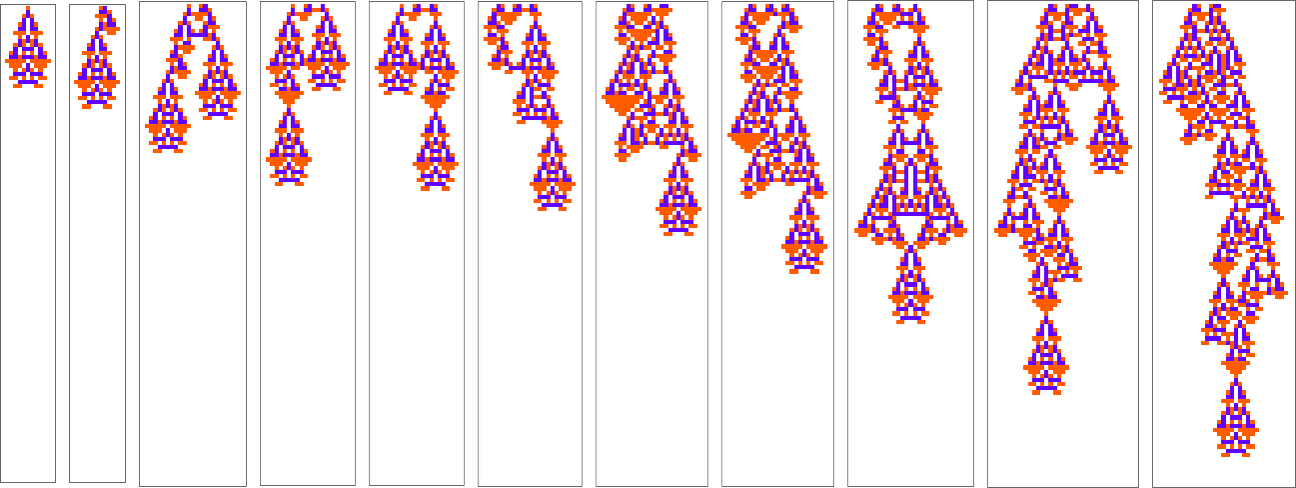
The sequence of lifetimes (“fitness values”) obtained in this process of adaptive evolution is
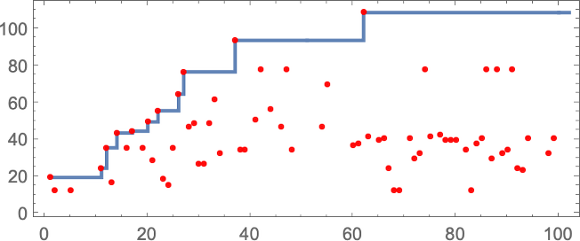
and the “breakthrough” initial conditions are:
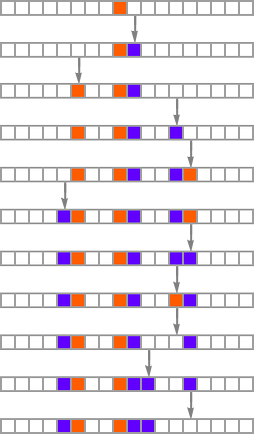
The basic setup is similar to what we’ve seen repeatedly in the adaptive evolution of rules rather than initial conditions. But one immediate difference is that, at least in the example we’ve just seen, changing initial conditions does not as obviously “introduce new ideas” for how to increase lifetime; instead, it gives more of an impression of just directly extending “existing ideas”.
So what happens more generally? Rules with k = 2, r = 1 tend to show either infinite growth or no growth—with finite lifetimes arising only from direct “erosion” of initial conditions (here for rules 104 and 164):

For k = 2, r = 2 rules the story is more complicated, even in the symmetric case. Here are the sequences of longest lifetime patterns obtained with all possible progressively wider initial conditions with various rules:
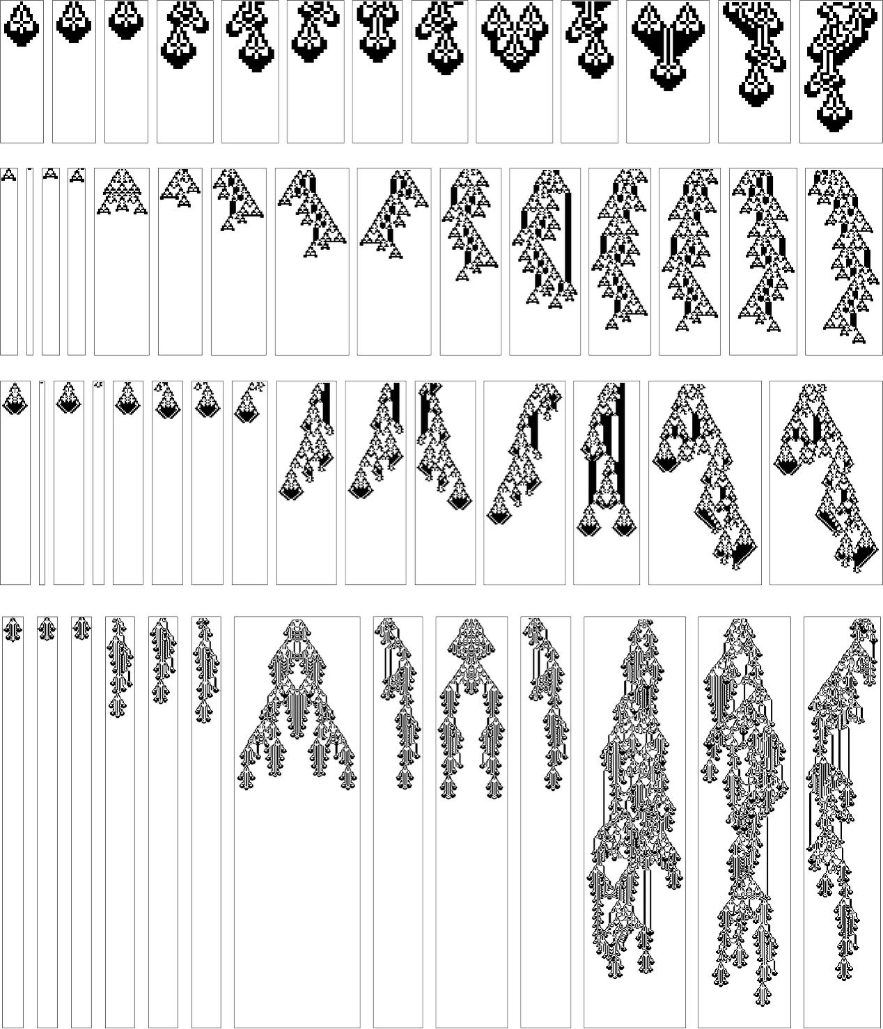
Again, there is a certain lack of “fundamentally new ideas” in evidence, though there are definitely “mechanisms” that get progressively extended with larger initial conditions. (One notable regularity is that the maximum lifetimes of patterns often seem roughly proportional to the width of initial condition allowed.)
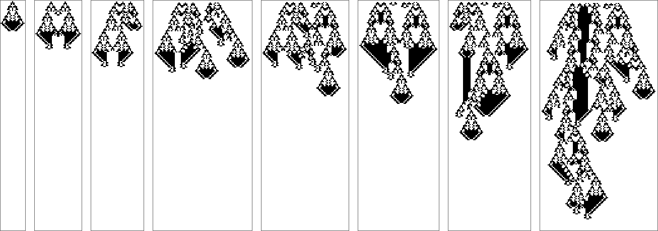
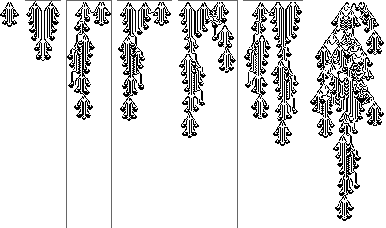
Can adaptive evolution “discover more”? Typically, when it’s just modifying initial conditions in a fixed region, it doesn’t seem so—again it seems to be more about “extending existing mechanisms” than introducing new ones:
2D Cellular Automata
Everything we’ve done so far has been for 1D cellular automata. So what happens if we go to 2D? In the end, the story is going to be very similar to 1D—except that the rule spaces even for quite minimal neighborhoods are vastly larger.
With k = 2 colors, it turns out that with a 5-cell neighborhood  one can’t “escape from the null rule” by single point mutations. The issue is that any single case one adds in the rule will either do nothing, or will lead only to unbounded growth. And even with a 9-cell neighborhood
  one can’t get rules that show growth that is neither limited nor infinite with a single-cell initial condition. But with a
  initial condition this is possible, and for example here is a sequence of phenotype patterns generated by adaptive evolution using lifetime as a fitness function:
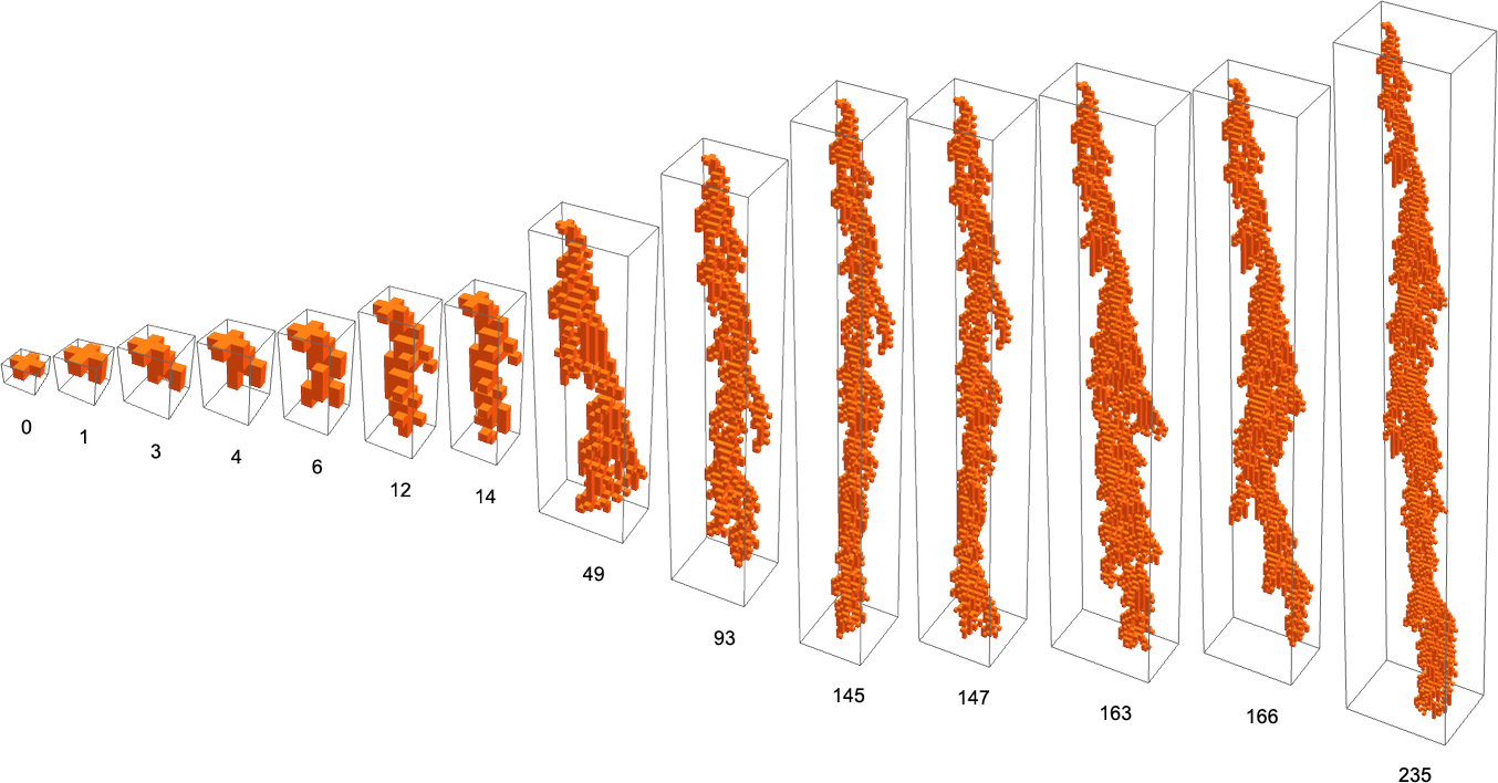
Here’s what these patterns look like when “viewed from above”:
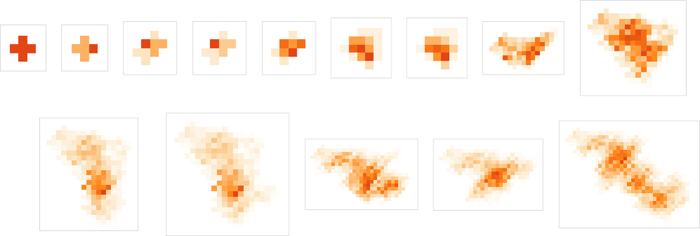
And here’s how the fitness progressively increases in this case:

There are a total of 2512 ≈ 10154 possible 9-neighbor rules, and in this vast rule space it’s easy for adaptive evolution to find rules with long finite lifetimes. (By the way, I’ve no idea what the absolute maximum “busy beaver” lifetime in this space is.)
Just as in 1D, there’s a fair amount of variation in the behavior one sees. Here are some examples of the “final rules” for various instances of adaptive evolution:
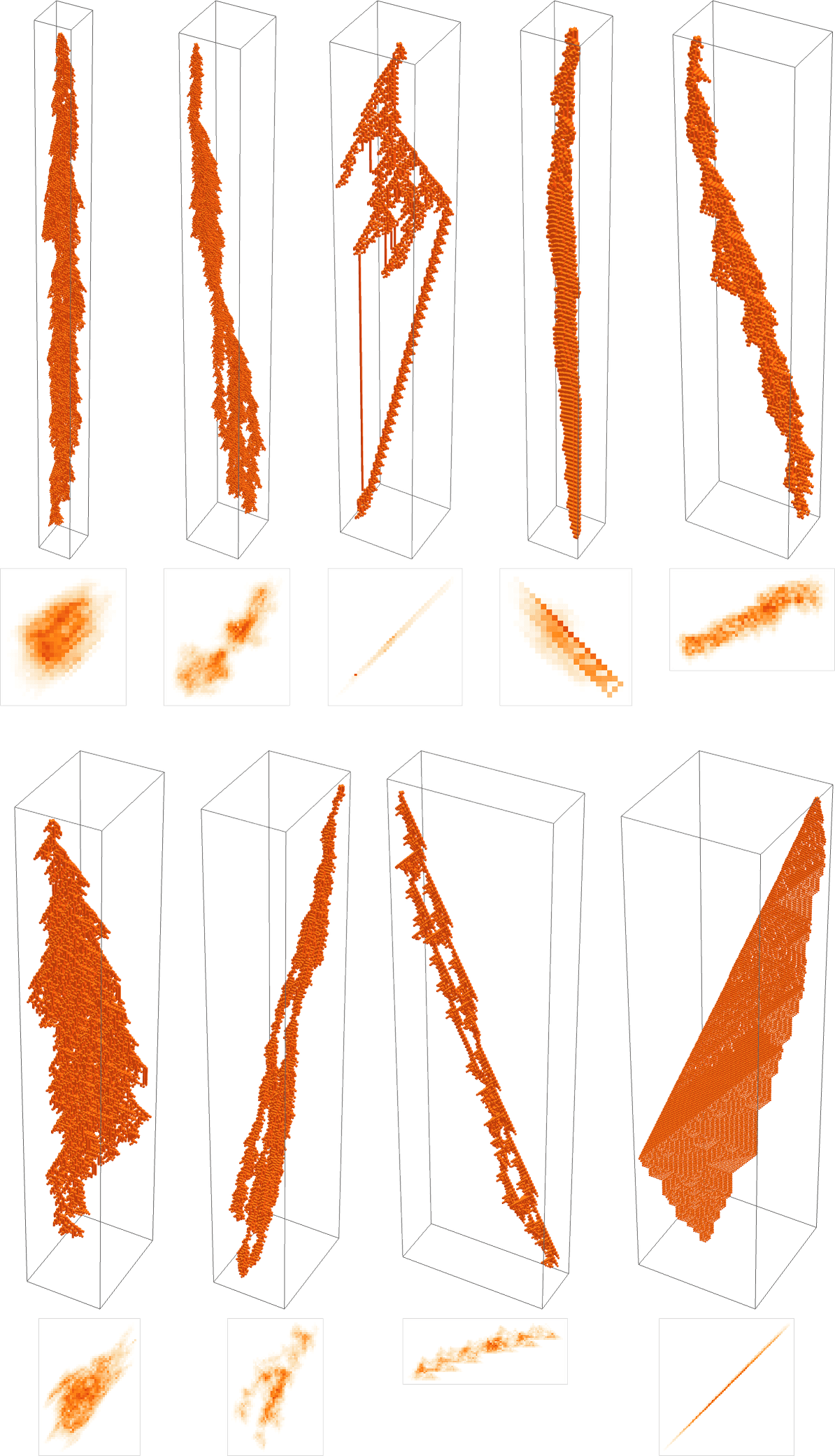
In a few cases one can readily “see the mechanism” for the lifetime—say associated with collisions between localized structures. But mostly, as in the other examples we’ve seen, there’s no realistic “narrative explanation” for how these rules achieve long yet finite lifetimes.
The Turing Machine Case
OK, so we’ve now looked at 2D as well as 1D cellular automata. But what about systems that aren’t cellular automata at all? Will we still see the same core phenomena of adaptive evolution that we’ve identified in cellular automata? The Principle of Computational Equivalence would certainly lead one to expect that we would. But to check at least one example let’s look at Turing machines.
Here’s a Turing machine with s = 3 states for its head, and k = 2 colors for cells on its tape:
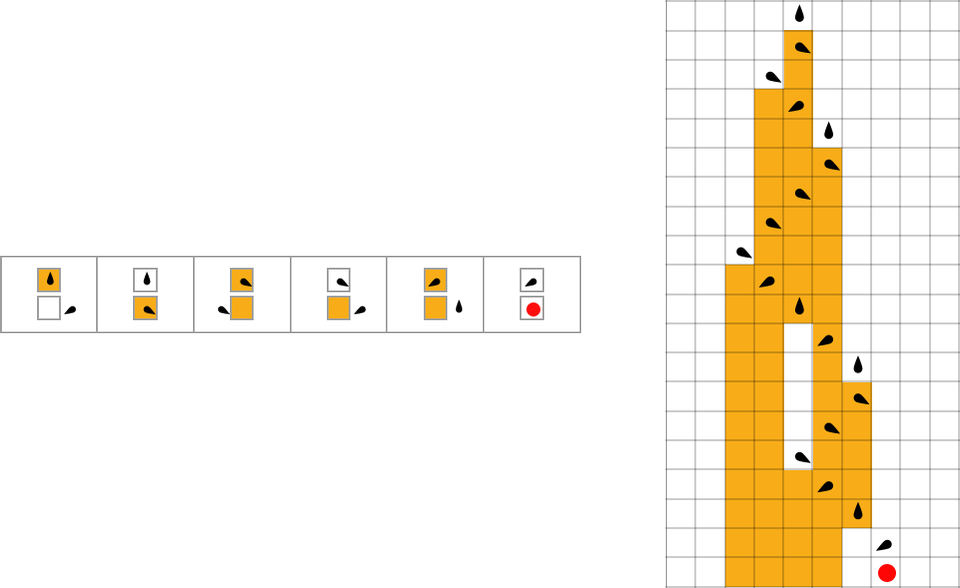
The Turing machine is set up to halt if it ever reaches a case in the rule where the output is  . Starting from a blank initial condition, this particular Turing machine halts after 19 steps.
So what happens if we try to adaptively evolve Turing machines with long lifetimes (i.e. that take many steps to halt)? Say we start from a “null rule” that halts in all cases, and then we make a sequence of single point mutations in the rule, keeping ones that don’t lead the Turing machine to halt in fewer steps than before. Here’s an example where the adaptive evolution eventually reaches a Turing machine that takes 95 steps to halt:
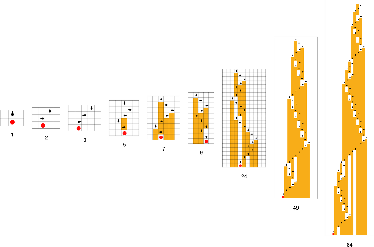
The sequence of (“breakthrough”) mutations involved here is
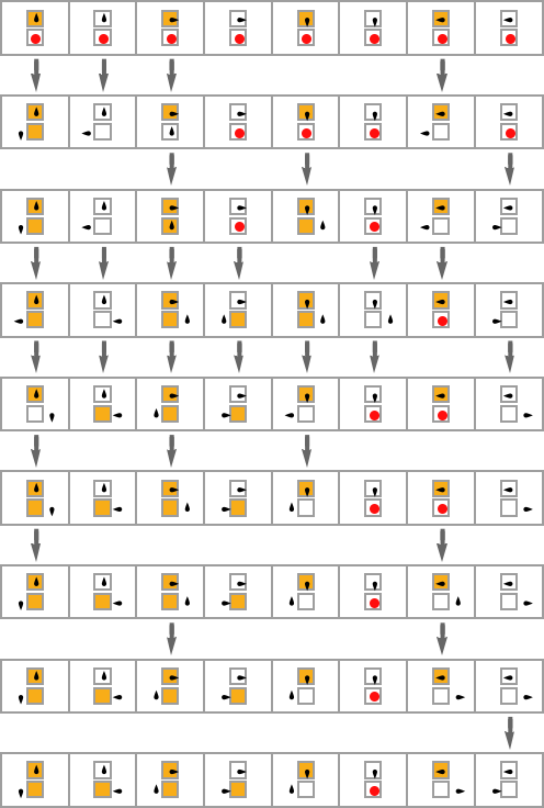
corresponding to a fitness curve of the form:
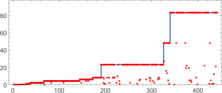
And, yes, all of this is very analogous to what we’ve seen in cellular automata. But one difference is that with Turing machines there are routinely much larger jumps in halting times. And the basic reason for this is just that Turing machines have much less going on at any particular step than typical cellular automata do—so it can take them much longer to achieve some particular state, like a halting state.
Here’s an example of adaptive evolution in the space of s = 3, k = 3 Turing machines—and in this case the final halting time is long enough that we’ve had to squash the image vertically (by a factor of 5):
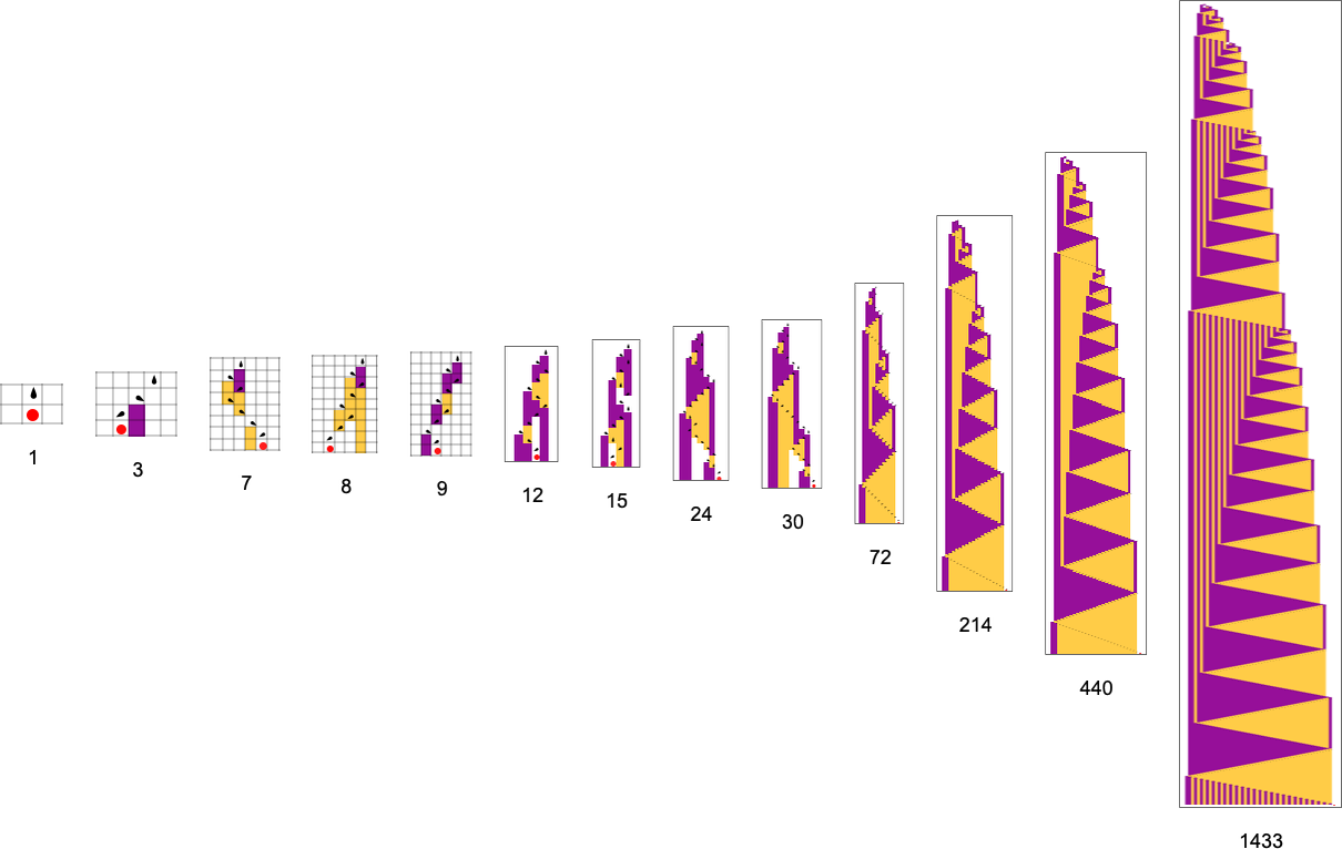
The fitness curve in this case is best viewed on a logarithmic scale:
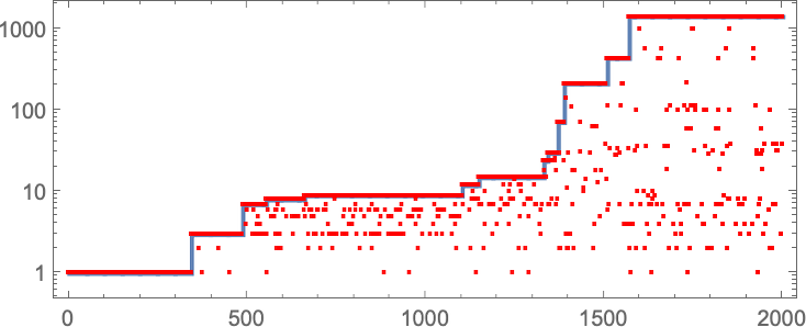
But while the largest-lifetime cellular automata that we saw above typically seemed to have very complex behavior, the largest-lifetime Turing machine here seems, at least on the face of it, to operate in a much more “systematic” and “mechanical” way. And indeed this becomes even more evident if we compress our visualization by looking only at steps on which the Turing machine head reverses its direction:
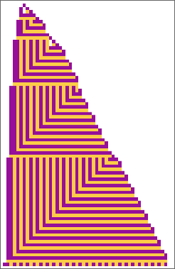
Long-lifetime Turing machines found by adaptive evolution are not always so simple, though they still tend to show more regularity than long-lifetime cellular automata:
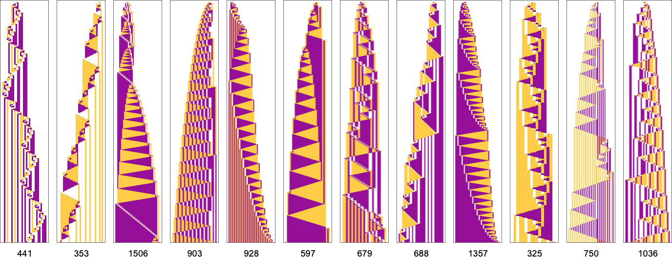
But—presumably because Turing machines are “less efficient” than cellular automata—the very longest possible lifetimes can be very large. It’s not clear whether rules with such lifetimes can be found by adaptive evolution—not least because even to evaluate the fitness function for any particular candidate rule could take an unbounded time. And indeed among s = 3, k = 3 rules the very longest possible is about 1017 steps—achieved by the rule

with the following “very pedantic behavior”:

So what about multiway evolution graphs? There are a total of 20,736 s = 2, k = 2 Turing machines with halting states allowed. From these there are 37 distinct finite-lifetime phenotypes:

Just as in other cases we’ve investigated, there are fitness-neutral sets such as:

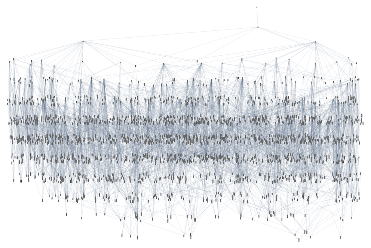
Taking just one representative from each of these 18 sets, we can then construct a multiway evolution graph for 2,2 Turing machines with lifetime as our fitness function:

Here’s the analogous result for 3,2 Turing machines—with 2250 distinct phenotypes, and a maximum lifetime of 21 steps (and the patterns produced by the machines just show by “slabs”):
We could pick other fitness functions (like maximum pattern width, number of head reversals, etc.) But the basic structure and consequences of adaptive evolution seem to work very much the same in Turing machines as in cellular automata—much as we expect from the Principle of Computational Equivalence.
Multiway Turing Machines
Ordinary Turing machines (as well as ordinary cellular automata) in effect always follow a single path of history, producing a definite sequence of states based on their underlying rule. But it’s also possible to study multiway Turing machines in which many paths of history can be followed. Consider for example the rule:

The ![]() case in this rule has two possible outcomes—so this is a multiway system, and to represent its behavior we need a multiway graph:
case in this rule has two possible outcomes—so this is a multiway system, and to represent its behavior we need a multiway graph:
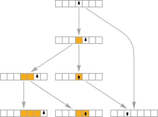
From a biological point of view, we can potentially think of such a multiway system as an idealized model for a process of adaptive evolution. So now we can ask: can we evolve this evolution? Or, in other words, can we apply adaptive evolution to systems like multiway Turing machines?
As an example, let’s assume that we make single point mutation changes to just one case in a multiway Turing machine rule:
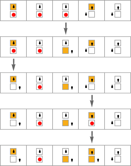
Many multiway Turing machines won’t halt, or at least won’t halt on all their branches. But for our fitness function let’s assume we require multiway Turing machines to halt on all branches (or at least go into loops that revisit the same states), and then let’s take the fitness to be the total number of nodes in the multiway graph when everything has halted. (And, yes, this is a direct generalization of our lifetime fitness function for ordinary Turing machines.)
So with this setup here are some examples of sequences of “breakthroughs” in adaptive evolution processes:

But what about looking at all possible paths of evolution for multiway Turing machines? Or, in other words, what about making a multiway graph of the evolution of multiway Turing machines?
Here’s an example of what we get by doing this (showing at each node just a single example of a fitness-neutral set):
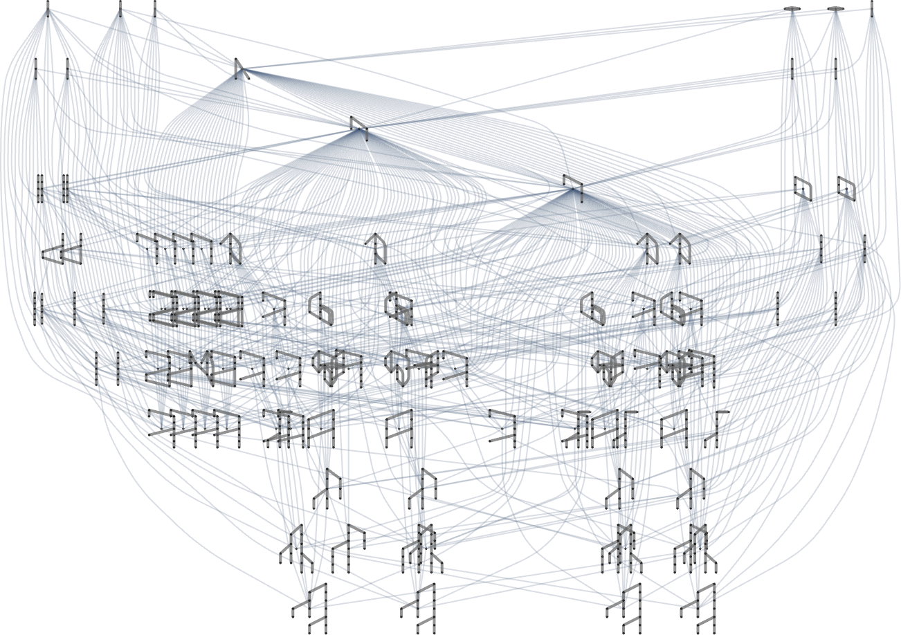
So what’s really going on here? We’ve got a multiway graph of multiway graphs. But it’s worth understanding that the inner and outer multiway graphs are a bit different. The outer one is effectively a rulial multiway graph, in which different parts correspond to following different rules. The inner one is effectively a branchial multiway graph, in which different parts correspond to different ways of applying a particular rule. Ultimately, though, we can at least in principle expect to encode branchial transformations as rulial ones, and vice versa.
So we can think of the adaptive evolution of multiway Turing machines as a first step in exploring “higher-order evolution”: the evolution of evolution, etc. And ultimately in exploring inevitable limits of recursive evolution in the ruliad—and how these might relate to the formation of observers in the ruliad.
Some Conclusions
What does all this mean for the foundations of biological evolution? First and foremost, it reinforces the idea of computational irreducibility as a dominant force in biology. One might have imagined that what we see in biology must have been “carefully sculpted” by fitness constraints (say imposed by the environment). But what we’ve found here suggests that instead much of what we see is actually just a direct reflection of computational irreducibility. And in the end, more than anything else, what biological evolution seems to be doing is to “recruit” lumps of irreducible computation, and set them up so as to achieve “fitness objectives”.
It is, as I recently discovered, very similar to what happens in machine learning. And in both cases this picture implies that there’s a limit to the kind of explanations one can expect to get. If one asks why something has the form it does, the answer will often just be: “because that’s the lump of irreducible computation that happened to be picked up”. And there isn’t any reason to think that there’ll be a “narrative explanation” of the kind one might hope for in traditional science.
The simplicity of models makes it possible to study not just particular possible paths of adaptive evolution, but complete multiway graphs of all possible paths. And what we’ve seen here is that fitness functions in effect define a kind of traversal order or (roughly) foliation for such multiway graphs. If such foliations could be arbitrarily complex, then they could potentially pick out specific outcomes for evolution—in effect successfully “sculpting biology” through the details of natural selection and fitness functions.
But the point is that fitness functions and resulting foliations of multiway evolution graphs don’t get arbitrarily complex. And even as the underlying processes by which phenotypes develop are full of computational irreducibility, the fitness functions that are applied are computationally bounded. And in effect the complexity that is perhaps the single most striking immediate feature of biological systems is therefore a consequence of the interplay between the computational boundedness of selection processes, and the computational irreducibility of underlying processes of growth and development.
All of this relies on the fundamental idea that biological evolution—and biology—are at their core computational phenomena. And given this interpretation, there’s then a remarkable unification that’s emerging.
It begins with the ruliad—the abstract object corresponding to the entangled limit of all possible computational processes. We’ve talked about the ruliad as the ultimate foundation for physics, and for mathematics. And we now see that we can think of it as the ultimate foundation for biology too.
In physics what’s crucial is that observers like us “parse” the ruliad in certain ways—and that these ways lead us to have a perception of the ruliad that follows core known laws of physics. And similarly, when observers like us do mathematics, we can think of ourselves as “extracting that mathematics” from the way we parse the ruliad. And now what we’re seeing is that biology emerges because of the way selection from the environment, etc. “parses” the ruliad.
And what makes this view powerful is that we have to assume surprisingly little about how selection works to still be able to deduce important things about biology. In particular, if we assume that the selection operates in a computationally bounded way, then just from the inevitable underlying computational irreducibility “inherited” from the ruliad, we immediately know that biology must have certain features.
In physics, the Second Law of thermodynamics arises from the interplay of underlying computational irreducibility of mechanical processes involving many particles or other objects, and our computational boundedness as observers. We have the impression that “randomness is increasing” because as computationally bounded observers we can’t “decrypt” the underlying computational irreducibility.
What’s the analog of this in biology? Much as we can’t expect to “say what happens” in a system that follows the Second Law, so we can’t expect to “explain by selection” what happens in a biological system. Or, put another way, much of what we see in biology is just the way it is because of computational irreducibility—and try as we might it won’t be “explainable” by some fitness criterion that we can describe.
But that doesn’t mean that we can’t expect to deduce “general laws of biology”, much as there are general laws about gases whose detailed structure follows the Second Law. And in what we’ve done here we can begin to see some hints of what those general laws might look like.
They’ll be things like bulk statements about possible paths of evolution, and the effect of changing the constraints on them—a bit like laws of fluid mechanics but now applied to the rulial space of possible genotypes. But if there’s one thing that’s clear it’s that the minimal model we’ve developed of biological evolution has remarkable richness and potential. In the past it’s been possible to say things about what amounts to the pure combinatorics of evolution; now we can start talking in a structured way about what evolution actually does. And in doing this we go in the direction of finally giving biology a foundation as a theoretical science.
There’s So Much More to Study!
Even though this is my second long piece about my minimal model of biological evolution, I’ve barely scratched the surface of what can be done with it. First and foremost there are many detailed connections to be made with actual phenomena that have been observed—or could be observed—in biology. But there are also many things to be investigated directly about the model itself—and in effect much ruliology to be done on it. And what’s particularly notable is how accessible a lot of that ruliology is. (And, yes, you can click any picture here to get the Wolfram Language code that generates it.) What are some obvious things to do? Here are few. Investigate other fitness functions. Other rule spaces. Other initial conditions. Other evolution strategies. Investigate evolving both rules and initial conditions. Investigate different kinds of changes of fitness functions during evolution. Investigate the effect of having a much larger rule space. Investigate robustness (or not) to perturbations.
In what I’ve done here, I’ve effectively aggregated identical genotypes (and phenotypes). But one could also investigate what happens if one in effect “traces every individual organism”. The result will be abstract structures that generalize the multiway systems we’ve shown here—and that are associated with higher levels of abstract formalism capable of describing phenomena that in effect go “below species”.
For historical notes see here »
Thanks
Thanks to Wolfram Institute fellows Richard Assar and Nik Murzin for their help, as well as to the supporters of the new Wolfram Institute initiative in theoretical biology. Thanks also to Brad Klee for his help. Related student projects were done at our Summer Programs this year by Brian Mboya, Tadas Turonis, Ahama Dalmia and Owen Xuan.
Since writing my first piece about biological evolution in March, I’ve had occasion to attend two biology conferences: SynBioBeta and WISE (“Workshop on Information, Selection, and Evolution” at the Carnegie Institution). I thank many attendees at both conferences for their enthusiasm and input. Curiously, before the WISE conference in October 2024 the last conference I had attended on biological evolution was more than 40 years earlier: the June 1984 Mountain Lake Conference on Evolution and Development.
